Machine Learning on Hyperspectral Scenes

This is where the workflow comes together. You have cleaned the cube, explored it visually, and measured it with your own index or use other indices. Now we let algorithms read the full spectrum of every pixel at once and organize the scene for us, first without any labels, then with a handful of examples you provide.
Important
All the concepts and theoretical foundations necessary to understand these tools and features of machine learning, except the supervised classification, have already been explained in the previous lessons of the Machine Learning Application module of this course. If you are reading these notebooks from the original TanagerSpec documentation repository, please visit the Hyperspectral Data Analysis course for those foundational explanations.
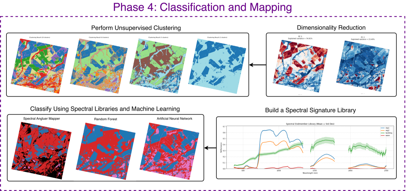
This lesson covers two complementary families (Phase 4 of the designed recipe):
- Unsupervised — let the data speak for itself, with no labels. We compress the spectrum with dimensionality reduction, then cluster pixels with similar spectra into groups.
- Supervised — you teach the model. You collect labelled example pixels into a spectral library, and a classifier learns to assign every pixel in the scene to one of your classes.
What You Will Learn
- Reduce dimensions (
.analysis.dim_reduction()): Compress 426 bands into a few informative components with PCA, MNF, or ICA. - Cluster (
.analysis.clustering()): Group pixels into spectral classes without any labels. - Build a spectral library (
.build_spectral_library()): Turn labelled training pixels into a reusable reference table of class spectra. - Classify (
.analysis.classify_scene()): Label every pixel using SAM, Random Forest, or a neural network—and export the result as a GeoTIFF for GIS.
Workspace Setup & TanagerSpec Initialization
Just like in previous lessons, this notebook is designed to run completely on its own.
Our first step is to set up our workspace and initialize TanagerSpec. The cell below will check your data/ folder for the scene (ortho_sr_scene.h5). If you're continuing straight from an earlier lesson, the script will detect your existing file and instantly skip the download. If you are jumping in fresh through Google Colab, don't worry, it will automatically fetch the data from the Open STAC catalog so we can get right to our machine-learning workflow.
## Unhide cell for package install if needed

# %pip install tanagerspec
# Standard library imports
from datetime import datetime               # For timestamping output folders
from pathlib import Path                    # For handling file and directory paths

# TanagerSpec package imports
from tanagerspec import download_scene      # Utility to download a Tanager scene
from tanagerspec import TanagerSpec         # Main class for Tanager hyperspectral data

# third party imports
import numpy as np
from scipy.stats import pearsonr
from sklearn.preprocessing import StandardScaler

# 1. Setup data and output directories
DATA_DIR = Path("data")
DATA_DIR.mkdir(parents=True, exist_ok=True)

timestamp = datetime.now().strftime("%Y%m%d_%H")   # unified format across the series
OUTPUT_DIR = Path(f"outputs_{timestamp}")
OUTPUT_DIR.mkdir(parents=True, exist_ok=True)

FIGURE_DIR = OUTPUT_DIR / "figures"
FIGURE_DIR.mkdir(parents=True, exist_ok=True)

# 2. Define scene parameters (clear agricultural scene, same as the Visualization lesson)
URL = "https://storage.googleapis.com/open-cogs/planet-stac/tanager1-release2-core-imagery/ortho_sr_hdf5/20250501_143138_87_4001_ortho_sr_hdf5.h5"
FILE_NAME = "ortho_sr_scene.h5"          # shared clear scene, reused across lessons
target_path = DATA_DIR / FILE_NAME

# 3. Smart download: only fetch if the file isn't already present
if target_path.exists():
    print(f"Scene already exists locally at: {target_path}. Skipping download.")
    TANAGER_SCENE_PATH = target_path
else:
    print("Local scene not found. Downloading from STAC...")
    TANAGER_SCENE_PATH = download_scene(URL, target_path)

# 4. Verify final path
if TANAGER_SCENE_PATH is not None and Path(TANAGER_SCENE_PATH).exists():
    print(f"Ready for analysis with scene: {TANAGER_SCENE_PATH}")
else:
    print("Error: Scene file is missing or download failed.")

# 5. Initialize TanagerSpec and prepare a clean cube for analysis
tanager_ortho_sr = TanagerSpec.from_file(TANAGER_SCENE_PATH)
tanager_ortho_sr.preprocess(masking=True, clipping=True)   # mask invalid/cloud pixels, clip to [0,1]

# 6. Denoise the scene (Optional)
tanager_ortho_sr.denoise(
    n_components=4,
)

print("TanagerSpec object initialized and preprocessed!")
Compress the Spectrum: .analysis.dim_reduction()
You already met this idea in the preprocessing lesson, where PCA reconstruction stripped noise from the cube.
TanagerSpec offers three engines:
- PCA (Principal Component Analysis): Components ordered by the variance they explain. Fast, general-purpose, and the usual first choice.
- MNF (Minimum Noise Fraction): A noise-adjusted cousin of PCA. It orders components by signal-to-noise ratio rather than raw variance, which often packs the useful structure into the first few components more cleanly—handy for noisy hyperspectral data.
- ICA (Independent Component Analysis): Seeks components that are statistically independent rather than merely uncorrelated, which can isolate distinct physical sources or materials.
Caution
When using ICA (Independent Component Analysis), be aware that it behaves differently from PCA and MNF. Unlike those methods, ICA does not order its components by variance or signal-to-noise ratio. The resulting components are not ranked, and the API returns only the results themselves without additional metadata or information about explained variance. Make sure you understand these differences when choosing ICA for your analysis.
The result is a (rows, cols, n_components) array—still a spatial image, just with far fewer, richer bands to feed into clustering or classification.
Parameter Reference
| Parameter | Type | Default | Description |
|---|---|---|---|
method |
str |
"PCA" |
Reduction engine: "PCA", "ICA", or "MNF" (case-insensitive). |
n_components |
int |
3 |
Number of components to retain. |
mask |
bool |
True |
If True, exclude invalid pixels using the scene masks before reducing. |
present_rgb |
str |
"true_color" |
RGB preset drawn behind the component visualization (e.g. "false_color_nir"). |
plot |
bool |
True |
Display the reduced components with the built-in visualizer. |
save_png |
str, False, or None |
None |
Path to save the figure; False / None skips saving. |
save_dpi |
int |
300 |
Resolution used when save_png is set. |
scatter_color_by |
str |
"Index" |
How to color the feature-space scatter: "component", "rgb", or "index". |
scatter_index, scatter_cmap |
str |
"NDVI", "RdYlGn" |
Index and colormap used when scatter_color_by="index". |
Important
scatter_color_by uses the same internal spectral-index calculation as calculate_index.
Choose the index name the same way: use IndexCatalog to find the available index names, then pass the desired name to scatter_index, for example "NDVI" or "EVI".
Returns
numpy.ndarray— the reduced cube of shape(rows, cols, n_components)(invalid pixels areNaN). Keep it in memory or save it yourself; export to GeoTIFF/NetCDF is not built into this method.
pca = tanager_ortho_sr.analysis.dim_reduction(
    method="MNF",                              # Replace it with "PCA" or "ICA"
    n_components=2,                            # Define the number of components
    present_rgb="false_color_nir",             # Define the RGB preset
    plot=True,                                 # Define if the plot is shown
    scatter_color_by="index",                  # Define how the scatter is colored
    scatter_index="NDVI",                      # Define the index used for coloring
    scatter_cmap="RdYlGn",                     # Define the colormap used for coloring
    save_png=FIGURE_DIR / "dim_reduction_plot.png"
)
Mix and Match: Compare a Reduced Component with a Spectral Index
Here is a point worth pausing on, because it changes how you can use everything you have learned so far. Every TanagerSpec analysis method hands you back a plain NumPy array, not a sealed object:
dim_reduction()→ a(rows, cols, n_components)cube,calculate_index()→ a(rows, cols)index map,clustering()→ a(rows, cols)label map.
Because these are ordinary arrays, you are never locked inside the library. The whole Python scientific stack, NumPy, SciPy, scikit-learn, pandas, is available to slice, scale, correlate, and recombine them, and you can freely mix the outputs of different TanagerSpec APIs to answer questions no single method answers on its own.
We will demonstrate this by asking a concrete question: does the data-driven first component (from dim_reduction) actually track the vegetation signal we measured with EVI (from calculate_index)? To find out, we take the two arrays, standardize them, compare them visually with compare_layers, and quantify the relationship with a correlation coefficient from SciPy.
# First Layer: a spectral index, straight from a TanagerSpec API
evi_array = tanager_ortho_sr.analysis.calculate_index(
    index_name="EVI",
    plot=False,
)

# Second Layer: the first reduced component from dim_reduction()
component1 = pca[:, :, 0]

# Standardize both arrays without flattening
scaler1 = StandardScaler()
component1_scaled = scaler1.fit_transform(component1)

scaler2 = StandardScaler()
evi_scaled = scaler2.fit_transform(evi_array)

# Mask out invalid (nan) values so correlation isn't affected
valid_mask = np.isfinite(component1_scaled) & np.isfinite(evi_scaled)
r, _ = pearsonr(component1_scaled[valid_mask], evi_scaled[valid_mask])
print(f"Pearson r between reduced component 1 and EVI: {r:.3f}")

# Visualization with compare_layers
comparison = tanager_ortho_sr.analysis.compare_layers(
    component1_scaled,
    evi_scaled,
    index1_name="Component 1 (scaled)",
    index2_name="EVI (scaled)",
    save_png=FIGURE_DIR / "comparison_PCA1_EVI.png",
)
Group Pixels Without Labels (Unsupervised Learning): .analysis.clustering()
Clustering is unsupervised: you do not tell the algorithm what anything is. You simply ask it to partition the pixels into a number of groups (n_clusters) so that pixels within a group have similar spectra and different groups look distinct. It is the natural way to get a first, label-free map of "what is spectrally different from what" across a scene.
You can cluster on the reduced components from Step 1 (recommended—faster and less noisy) by setting dr_method, or on all 426 bands at once with dr_method=None. Two algorithms are available:
- K-Means: Partitions pixels into
kcompact groups around cluster centres. Fast and intuitive; assumes roughly round, similarly sized clusters. - GMM (Gaussian Mixture Model): Fits overlapping Gaussian "blobs," allowing clusters of different shapes and sizes and softer boundaries between them.
The output is a 2D label map (one integer per pixel). Remember that cluster IDs are arbitrary—the algorithm finds groups, not meanings. Interpreting which cluster is water, vegetation, or soil is your job, typically by comparing the cluster map against an RGB composite or known signatures.
Parameter Reference
| Parameter | Type | Description |
|---|---|---|
dr_method |
str or None |
None clusters the full band space. "PCA", "ICA", or "MNF" reduces to n_components first, then clusters in that feature space. |
n_components |
int or None |
Number of reduced dimensions when dr_method is set; use None when dr_method=None. |
clustering_method |
str |
"KMEANS" or "GMM" (Gaussian mixture). |
n_clusters |
int |
Number of clusters / mixture components to form. |
present_rgb |
str |
RGB preset drawn behind the cluster map (default "true_color"). |
plot |
bool |
If True, show the cluster map beside the RGB context. |
save_geotiff |
str or None |
Write a one-band integer label GeoTIFF (uses the scene's grid_info when available). |
save_png |
str or None |
Path to save the figure. |
save_dpi |
int |
DPI for save_png (default 300). |
**kwargs |
— | Forwarded to the clustering model (e.g. random_state, n_init, max_iter; GMM covariance_type, reg_covar). |
Returns
numpy.ndarray— a 2D(rows, cols)map of integer cluster labels; invalid pixels are-9999(shown as gaps in the plot).
clustered_array = tanager_ortho_sr.analysis.clustering(
    dr_method="PCA",                  # Dimension reduction: "PCA", "ICA", "MNF", or None for all bands
    n_components=3,                   # Number of reduced dimensions (if using dr_method)
    clustering_method="KMEANS",       # Clustering algorithm: "KMEANS" or "GMM"
    n_clusters=5,                     # Number of clusters to identify
    random_state=42,                  # For reproducible labels
    save_png=FIGURE_DIR / "clustering_plot.png",        # Save the cluster plot as PNG
    save_dpi=300,                                     # PNG resolution
    save_geotiff=OUTPUT_DIR / "ortho_clustering.tif",  # Export clusters as GeoTIFF
    # present_rgb="false_color_nir",                   # Optionally set RGB background
)
Teach the Model: .build_spectral_library()
Clustering finds groups but cannot name them. To produce a map of named classes, water, vegetation, buildings, we switch to supervised learning, which needs labelled examples.
build_spectral_library() is how you provide them. For each class you give one or more (col, row) locations, and the tool cuts a small spatial window around each point and collects the valid spectra inside it. Averaging over a window rather than trusting a single pixel stabilizes the signature against noise and captures a little of the natural variability within the class.
It returns two things: a dictionary of per-class mean ± standard-deviation spectra (used directly by the SAM classifier), and a tidy training table, one row per sampled spectrum, one column per wavelength, plus a Label column—ready for the Random Forest and neural-network classifiers.
Important
The quality of everything downstream depends on these examples being pure and representative, so choose your training pixels carefully.
Warning
Coordinate order is (col, row) = (x, y) here — the transpose of the (row, col) order that .plot.hunt_pixels() and .plot.pixel_spectra() use. When you read a location off hunt_pixels (which reports row, col), swap the two numbers before passing it to build_spectral_library. A swapped coordinate won't raise an error; it will just sample the wrong pixel, so double-check each target on the RGB context panel the tool draws.
Parameter Reference
| Parameter | Type | Default | Description |
|---|---|---|---|
targets |
dict |
— | Class name → a single (col, row) tuple or a list of (col, row) tuples for several training pixels per class. |
window_size |
int |
5 |
Odd-sized square window (e.g. 5×5) averaged around each point over valid pixels. |
plot |
bool |
True |
Show the mean ± std spectra alongside the RGB context with your points marked. |
export_csv |
str or None |
None |
Path to save the training table as CSV. |
save_png |
str or None |
None |
Path to save the library figure. |
Returns
(library_means, df_library)library_means—dictmapping each class →{"mean": 1D array, "std": 1D array}.df_library— apandas.DataFramewith one row per extracted spectrum, per-wavelength columns, and aLabelcolumn.
# run hunt_pixels to get the coordinates of the training pixels
# tanager_ortho_sr.plot.hunt_pixels()
library_stats, df_training = tanager_ortho_sr.build_spectral_library(
    # class name -> (col, row), or a list of (col, row) tuples for several training pixels.
    # NOTE: this is (col, row) = (x, y) -- the TRANSPOSE of hunt_pixels' (row, col).
    # Verify/adjust each point with tanager_ortho_sr.plot.hunt_pixels() and swap the
    # two numbers (hunt_pixels reports row, col) before pasting them here.
    targets={
        "veg1":     [(369, 364)],
        "veg2":     (188, 287),
        "building": (294, 509),
        "water":    (518, 451),
    },
    window_size=5,                # 5x5 window (25 pixels) averaged around each point
    export_csv=OUTPUT_DIR / "ml_spectral_training_set.csv",
)
Label Every Pixel (Supervised Learning): .analysis.classify_scene()
With a spectral library in hand, classify_scene() assigns every pixel in the scene to one of your classes. Three methods are offered, trading physical interpretability for flexibility:
- SAM (Spectral Angle Mapper): Treats each pixel's spectrum as a vector and measures the angle between it and each class-mean spectrum; the smallest angle wins (if it falls below
sam_threshold). Because it compares shape rather than magnitude, SAM is largely insensitive to brightness differences such as illumination and shadow—a physically intuitive baseline with very few parameters. - Random Forest (RF): An ensemble of decision trees trained on your labelled table. It learns flexible, non-linear boundaries between classes and is robust and hard to over-tune—usually the strongest general-purpose choice.
- Neural Network (NN): A multilayer perceptron that can model the most complex boundaries, at the cost of more data and tuning (
nn_hidden_layer_sizes,nn_max_iter).
Each returns a 2D map of class labels you can plot over an RGB context and export as a GeoTIFF.
Note
A classified map always looks convincing, but accuracy depends on the training pixels. Validate results against independent reference points before drawing conclusions, and treat sparse or unrepresentative training data as the most likely source of error.
Parameter Reference
| Parameter | Type | Default | Description |
|---|---|---|---|
method |
str |
— | "SAM", "RF", or "NN". |
library_means |
dict |
None |
SAM only. Class name → 1D mean spectrum. Accepts library_stats directly (it reads each class's "mean"). |
df_training |
DataFrame |
None |
RF / NN only. The training table from build_spectral_library (wavelength columns + Label). |
sam_threshold |
float |
0.15 |
SAM. Max spectral angle (radians) to accept a match; larger angles are left unclassified. |
rf_estimators |
int |
100 |
RF. Number of trees. |
confidence_threshold |
float or None |
None |
RF / NN. Minimum class probability; lower-confidence pixels become Unclassified (0). |
nn_hidden_layer_sizes |
tuple |
(100,) |
NN. Hidden-layer sizes, e.g. (10, 10) for two layers. |
nn_max_iter |
int |
500 |
NN. Max training iterations. |
nn_early_stopping |
bool or None |
None |
NN. Toggle MLP early stopping; None lets the backend decide. |
present_rgb |
str |
"true_color" |
RGB preset behind the classification map. |
plot |
bool |
True |
Show the classification map over the RGB context. |
save_geotiff / save_png |
str or None |
None |
Optional paths for a label GeoTIFF and/or the figure. |
Returns
numpy.ndarray— a 2D(rows, cols)map of integer class labels, where-9999is NoData,0is Unclassified, and1..Nare your classes (in the order shown by the visualizer's legend).
# Prepare the mean spectra for each class, required for the SAM algorithm
pure_means = {k: v["mean"] for k, v in library_stats.items()}

# Set the SAM threshold: the maximum spectral angle (in radians) to accept a match; larger angles are left unclassified
sam_threshold = 0.1

# Classify every pixel in the scene using the Spectral Angle Mapper (SAM) method.
# This compares the spectrum at each pixel to the mean spectrum of every class, assigning the closest match.
# Outputs a GeoTIFF where each pixel is labelled with its predicted class.
sam_prediction = tanager_ortho_sr.analysis.classify_scene(
    method="SAM",                             # Use the SAM algorithm for classification
    library_means=pure_means,                 # Pass the class mean spectra
    sam_threshold=sam_threshold,              # Specify the SAM threshold
    present_rgb="false_color_nir",            # Use NIR false color as background for visualization
    save_geotiff=OUTPUT_DIR / "ortho_sam_classification.tif",  # Save the predicted label map as GeoTIFF
)
# Classify every pixel in the scene using the Random Forest (RF) algorithm.
# This method uses the training DataFrame produced earlier to train a collection of decision trees.
# Each pixel is labeled based on the class predictions of the trained RF model.
rf_prediction = tanager_ortho_sr.analysis.classify_scene(
    method="RF",                                    # Use the Random Forest algorithm
    df_training=df_training,                        # Training data (features + labels)
    rf_estimators=100,                              # Number of trees in the forest
    present_rgb="false_color_nir",                  # Use NIR false color as the background for visualization
    confidence_threshold=0.6,                       # Only classify pixels with at least 60% class probability
    save_geotiff=OUTPUT_DIR / "ortho_rf_classification.tif",  # Save the classification result as a GeoTIFF
)
# Classify every pixel in the scene using a Neural Network (NN) classifier.
# - This method uses a Multi-layer Perceptron (MLP) trained on the earlier training dataframe.
# - Each pixel’s spectrum is fed to the trained NN; pixels are labelled with their predicted class.
# - Only confidently classified pixels (≥ 50% probability) receive a class label, otherwise "Unclassified".
# - Two hidden layers are used (10, 10, 5 neurons), with up to 1000 training iterations.
# - The result is visualized over a NIR false color background,
#   and saved as both a PNG and a GeoTIFF.
nn_predictions = tanager_ortho_sr.analysis.classify_scene(
    method="NN",                                        # Use Neural Network classification
    df_training=df_training,                            # Training dataset (features + labels)
    nn_hidden_layer_sizes=(10, 10, 5),                  # Three hidden layers: 10, 10, and 5 neurons
    nn_max_iter=1000,                                   # Maximum training iterations
    present_rgb="false_color_nir",                      # NIR false color as visualization background
    confidence_threshold=0.5,                           # Minimum classification confidence (50%)
    nn_early_stopping=False,                            # Do not use early stopping in NN training
    plot=True,                                          # Display classification results
    save_png=FIGURE_DIR / "nn_classification.png",      # Save PNG visualization
    save_geotiff=OUTPUT_DIR / "nn_predictions.tif",     # Save predicted labels as GeoTIFF
)
Congratulations — You've Completed the TanagerSpec Crash Course!
You have taken a Tanager-1 scene the full distance: from a raw HDF5-EOS file to a cleaned cube, GIS-ready exports, true- and false-colour composites, spectral signatures, catalog and custom indices, and finally clustered and classified maps backed by machine learning.
More importantly, you have seen how the pieces connect into a workflow, how preprocessing protects your statistics, how visualization and indices guide where to look, and how dimensionality reduction feeds clustering and classification. You can now repeat this end-to-end recipe on your own scenes, or remix the tools to answer the questions that matter to your research.
Best of luck with your hyperspectral explorations!