Architecture
TanagerSpec is not just a bag of functions — it is a deliberately designed system. The guiding idea is that once you learn one part, the rest feels familiar. This page explains the design philosophy, walks through the package architecture, and traces how data and control flow from a raw file to a finished product.
Design philosophy
One object owns the scene
You load a scene once into a single TanagerSpec instance, and everything — preprocessing, plotting, analysis, export — is discoverable on that one object. There is no juggling of helper functions, format converters, and global state. The
scene is the API.
from tanagerspec import TanagerSpec

scene = TanagerSpec.from_file("scene.h5")
# from here on, your whole analysis is `scene.<something>`
Accessor namespaces that read like English
Capabilities are grouped into three intuitive namespaces, so the code says what it does:
scene.plot.*          →  see it          (rgb, bands_gallery, pixel_spectra, hunt_pixels, …)
scene.analysis.*      →  compute on it   (calculate_index, dim_reduction, clustering, classify_scene, …)
scene.convert_to.*    →  take it out     (geotiff, envi_bil, xarray)
This separation of concerns keeps the surface tidy and makes the package tab-discoverable — type scene.plot. in a notebook and the right tools are right there. For the complete list of methods and their parameters, see the API Reference.
A consistent grammar across every method
Methods follow the same predictable shape: analysis options first, presentation controls second.
- Analysis options —
preset,n_components,index_name,mask_threshold, … - Presentation controls —
plot=,save_png=,save_geotiff=
Learn one method and you can guess the rest. Want a figure? plot=True. Want it saved? save_png="out.png". Want a GIS layer? save_geotiff="out.tif". The same RGB preset system (true_color, false_color_nir, false_color_swir, false_color_urban) is reused everywhere — in scene.plot.rgb, ROI tools, and index context maps alike.
Composable by design — data flows as plain arrays
Index maps, PCA components, cluster labels, and classification maps are all just 2-D / 3-D NumPy arrays. Because the package speaks a common currency, the same tools work on any result. Comparing an NDVI map to a custom index, or to a PCA component, uses the exact same calls you already know (for example scene.analysis.compare_layers).
Stateful and self-aware
A TanagerSpec object tracks its own state. Calling scene.info() reports the current product type, cube shape, band count, dropped bands, and whether the cube has been denoised. Key operations such as preprocess() and denoise() work in place to save memory, and denoise() is idempotent — it refuses to run twice on the same cube. These safeguards help you avoid accidentally repeating work or losing track of your data.
GIS-native by default
Every map is one argument away from your GIS. Clustering and classification accept save_geotiff=, and scene.convert_to bridges to GeoTIFF, ENVI-BIL, and xarray/NetCDF, so results drop straight into QGIS, ArcGIS, ENVI, or any xarray workflow.
Package architecture
The diagram below is the class-level architecture of tanagerspec. It shows the domain models, the loader, the central scene object, and the three namespaces.
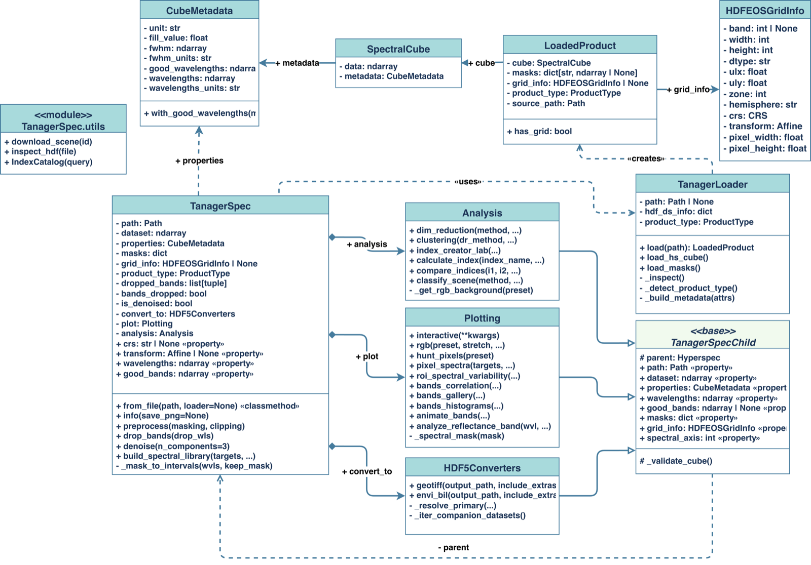
Reading the diagram from the data inward:
-
Domain models (frozen dataclasses,
core/models.py) —CubeMetadataholds per-band metadata (wavelengths, FWHM, units, and the good-band mask);SpectralCubebundles the NumPydataarray with itsCubeMetadata; andLoadedProductis the complete output of a load: theSpectralCube, per-pixelmasks, an optionalgrid_info, the detectedproduct_type, and thesource_path.HDFEOSGridInfo(io/tanager_grid.py) carries the CRS and affine transform for orthorectified products. These models are frozen to prevent accidental shared-state mutation; updates go through helpers such asCubeMetadata.with_good_wavelengths(). -
TanagerLoader(io/) — opens the HDF5-EOS file, introspects shape and dtype, detects the product type, and creates aLoadedProduct. It is the only sensor-specific component; everything downstream consumes the standardized models. -
TanagerSpec(the scene object) — wraps exactly oneLoadedProduct. It exposes the mutable spectral cube asdataset, surfaces metadata through properties (wavelengths,good_bands,crs,transform), and tracks processing state (dropped_bands,bands_dropped,is_denoised). Its core methods —info(),preprocess(),drop_bands(),denoise(),build_spectral_library()— act directly on the cube. -
The three namespaces —
Plotting(scene.plot),Analysis(scene.analysis), andHDF5Converters(scene.convert_to) are attached to the scene at construction. They are thin facades: each validates inputs and forwards to backend functions inviz/,analysis/, andconverters/. -
TanagerSpecChild(base class,core/child_base.py) — every namespace inherits from it. It holds a reference to theparentscene and re-reads the parent's currentdataset,wavelengths,good_bands,masks, andgrid_infoon each call. This is why processing methods can mutate the parent in place and the namespaces immediately see the latest state, with no arguments to thread through. -
Module-level utilities (
utils/) —download_scene(),inspect_hdf(), andIndexCatalogare re-exported at the top level oftanagerspecand can be used without constructing a scene.
Data and control flow
A typical analysis moves through the system like this:
flowchart TD
    hdf["HDF5-EOS file"] --> loader["TanagerLoader (io)"]
    loader -->|creates| product["LoadedProduct (core.models)"]
    product --> scene["TanagerSpec"]
    scene --> process["preprocess / drop_bands / denoise (process) — in place"]
    scene --> plot["scene.plot.*"]
    scene --> analysis["scene.analysis.*"]
    scene --> convert["scene.convert_to.*"]
    plot --> viz["viz/ backends"]
    analysis --> analysisBackends["analysis/ backends (exploration, indices, unsupervised, classification)"]
convert --> converters["converters/ (GeoTIFF, ENVI-BIL, xarray)"]TanagerSpec.from_file(path)asksTanagerLoaderto read the file and return a frozenLoadedProduct.- The scene wraps that product and exposes the cube as a mutable NumPy array.
- Optional in-place processing (
preprocess,drop_bands,denoise) updates the cube and the good-band mask on the scene. - Visualization, analysis, and export are invoked through the namespaces, which read the scene's current state via
TanagerSpecChildand delegate to the backend modules.
For the contributor's view of which file holds each of these pieces — and where to add new ones — continue to Source Layout. For the in-memory cube contract and xarray export conventions, see Conventions.