Calculating and Comparing Spectral Indices with TanagerSpec¶

With our hyperspectral data cleaned and our visualization skills established, we are ready to transition from exploratory viewing to targeted quantitative analysis. In this lesson, we will execute Phase 3 of our hyperspectral analysis recipe: Spectral Index Development.

Spectral indices are mathematical equations applied across targeted narrow bands to amplify the signal of a particular surface material, such as vegetation biomass, water turbidity, or burn severity, while suppressing background noise and illumination effects.

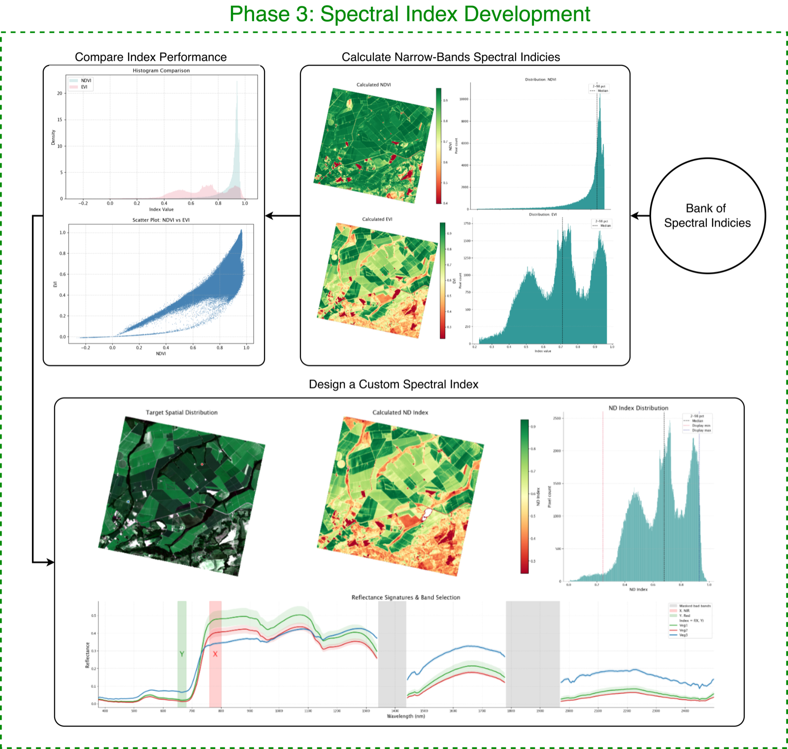
Rather than forcing you to manually research formulas, match nanometer wavelengths, and slice array bands by hand, TanagerSpec features a highly optimized quantitative index engine powered by an extensive built-in library.

What You Will Learn¶

In this lesson, you will learn how to extract quantitative thematic layers from your data cube. Specifically, we will cover how to:

• Query the Built-in Database (IndexCatalog): Search and explore registered indices across diverse application domains (like vegetation, water, burn, and urban) to review exact formulas, target wavelengths, and academic citations directly in your console.
• Calculate Thematic Layers (.analysis.calculate_index): Automatically map complex index math to your preprocessed scene to generate optimized 2D NumPy arrays, apply lower-bound masks to drop background noise, and render polished maps over contextual RGB underlays.
• Compare Index Performance (.analysis.compare_layers): Perform side-by-side quantitative evaluations of two different indices using pixel-by-pixel scatter plots and overlaid density distributions to analyze environmental sensitivity, linear correlations, and saturation limits.

Let’s re-establish our clean workspace directories and start exploring the index catalog!

Workspace Setup & TanagerSpec Initialization¶

Just as in our previous modules, this notebook is fully self-contained and designed to run independently.

Our first step is to establish our clean workspace and initialize TanagerSpec. The execution cell below will scan your local data/ directory for our target hyperspectral scene (ortho_sr_scene.h5). If you are continuing your work directly from Lessons 1, 2, or 3, the script will detect your existing file and instantly bypass the download process.

If you are jumping into this lesson fresh or running the notebook via Google Colab, don't worry! The setup script will automatically fetch the required data cube from the Open STAC catalog so we can dive right into our analysis workflow.

In [ ]:

## Unhide cell for package install if needed

# %pip install tanagerspec

## Unhide cell for package install if needed # %pip install tanagerspec

In [ ]:

# Standard library imports
from datetime import datetime               # For timestamping output folders
from pathlib import Path                    # For handling file and directory paths

# TanagerSpec package imports
from tanagerspec import download_scene      # Utility function to download a Tanager scene
from tanagerspec import TanagerSpec         # Main class for interacting with Tanager hyperspectral data

# third party imports
import matplotlib.pyplot as plt

# 1. Setup Data and Output Directories
DATA_DIR = Path("data")
DATA_DIR.mkdir(parents=True, exist_ok=True)

timestamp = datetime.now().strftime("%Y%m%d_%H")
OUTPUT_DIR = Path(f"outputs_{timestamp}")
OUTPUT_DIR.mkdir(parents=True, exist_ok=True)

# Figure directory
FIGURE_DIR = OUTPUT_DIR / "figures"
FIGURE_DIR.mkdir(parents=True, exist_ok=True)

# 2. Define Scene Parameters
URL = 'https://storage.googleapis.com/open-cogs/planet-stac/tanager1-release2-core-imagery/ortho_sr_hdf5/20250501_143138_87_4001_ortho_sr_hdf5.h5'
FILE_NAME = "ortho_sr_scene.h5"
target_path = DATA_DIR / FILE_NAME

# 3. Smart Download: Check if file exists before downloading
if target_path.exists():
    print(f"Scene already exists locally at: {target_path}. Skipping download.")
    TANAGER_SCENE_PATH = target_path
else:
    print("Local scene not found. Downloading from STAC...")
    TANAGER_SCENE_PATH = download_scene(
        URL,          # URL of the HDF5 file to download 
        target_path   # Destination path to save the file
    )

# 4. Verify Final Path
if TANAGER_SCENE_PATH is not None and Path(TANAGER_SCENE_PATH).exists():
    print(f"Ready for preprocessing with scene: {TANAGER_SCENE_PATH}")
else:
    print("Error: Scene file is missing or download failed.")

# 5. Initialize the TanagerSpec object using the verified scene path
tanager_ortho_sr = TanagerSpec.from_file(TANAGER_SCENE_PATH)

# 6. Denoise the scene (Optional)
tanager_ortho_sr.denoise(
    n_components=4,
)

print("TanagerSpec object successfully initialized!")

# Standard library imports from datetime import datetime # For timestamping output folders from pathlib import Path # For handling file and directory paths # TanagerSpec package imports from tanagerspec import download_scene # Utility function to download a Tanager scene from tanagerspec import TanagerSpec # Main class for interacting with Tanager hyperspectral data # third party imports import matplotlib.pyplot as plt # 1. Setup Data and Output Directories DATA_DIR = Path("data") DATA_DIR.mkdir(parents=True, exist_ok=True) timestamp = datetime.now().strftime("%Y%m%d_%H") OUTPUT_DIR = Path(f"outputs_{timestamp}") OUTPUT_DIR.mkdir(parents=True, exist_ok=True) # Figure directory FIGURE_DIR = OUTPUT_DIR / "figures" FIGURE_DIR.mkdir(parents=True, exist_ok=True) # 2. Define Scene Parameters URL = 'https://storage.googleapis.com/open-cogs/planet-stac/tanager1-release2-core-imagery/ortho_sr_hdf5/20250501_143138_87_4001_ortho_sr_hdf5.h5' FILE_NAME = "ortho_sr_scene.h5" target_path = DATA_DIR / FILE_NAME # 3. Smart Download: Check if file exists before downloading if target_path.exists(): print(f"Scene already exists locally at: {target_path}. Skipping download.") TANAGER_SCENE_PATH = target_path else: print("Local scene not found. Downloading from STAC...") TANAGER_SCENE_PATH = download_scene( URL, # URL of the HDF5 file to download target_path # Destination path to save the file ) # 4. Verify Final Path if TANAGER_SCENE_PATH is not None and Path(TANAGER_SCENE_PATH).exists(): print(f"Ready for preprocessing with scene: {TANAGER_SCENE_PATH}") else: print("Error: Scene file is missing or download failed.") # 5. Initialize the TanagerSpec object using the verified scene path tanager_ortho_sr = TanagerSpec.from_file(TANAGER_SCENE_PATH) # 6. Denoise the scene (Optional) tanager_ortho_sr.denoise( n_components=4, ) print("TanagerSpec object successfully initialized!")

Now that we've set up our workspace and are ready to calculate indices, it's time to introduce you to the IndexCatalog in TanagerSpec, which provides a bank of indices for different domains!

Exploring Spectral Formulas with the IndexCatalog¶

For the general call shape (object.accessor.method, assigning outputs, export kwargs), see Lesson 15 — How TanagerSpec Method Calls Are Structured.

With hundreds of spectral indices published across remote sensing literature, keeping track of exact formulas, required wavelengths, and source references can be tedious. To solve this, TanagerSpec integrates the widely recognized Awesome Spectral Indices library, harmonizing its extensive bank of formulas specifically for Tanager-1's hyperspectral bands via the IndexCatalog.

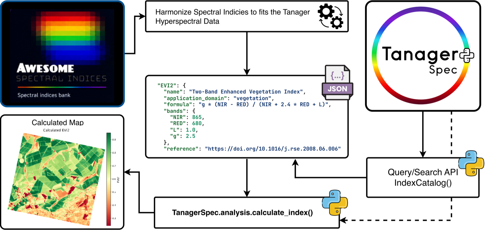
The IndexCatalog acts as an interactive console helper. It reads the underlying harmonized database and formats the information cleanly in your terminal, acting as the bridge between mathematical theory and your automated spatial mapping.

💡 Core Concept: Visual Reference Only The IndexCatalog is strictly a visual reference tool designed to print formatted diagnostic text to your console. It does not return Python dictionaries or lists for you to iterate over in code. Use it to explore capabilities, verify formula math, and find the exact index_name string you need to pass into the .analysis.calculate_index() engine later.

Available Application Domains¶

The catalog categorizes spectral formulas into distinct environmental and physical application domains to streamline your search:

• vegetation: Assess canopy health, greenness, chlorophyll content, and leaf area.
• water: Track open water boundaries, turbidity, and drought metrics.
• soil: Highlight bare soil, biological crusts, and mineral composition.
• burn: Quantify fire boundaries and post-fire burn severity.
• snow: Map snow cover, ice differentiation, and grain size.
• urban: Isolate built environments, impervious surfaces, and roads.
• clouds: Detect thick cloud cover and thin cirrus interference.

Querying the Catalog in Code¶

You can follow the steps below to initialize the catalog and explore how to navigate domains, inspect specific categories, view deep-dive index details, and perform keyword searches directly within your notebook:

from tanagerspec import IndexCatalog

# 1. Initialize the Index Catalog helper
cat = IndexCatalog()

# 2. View all available application domains
print("--- ALL APPLICATION DOMAINS ---")
cat.print_domains()

# 3. List all registered indices within a specific domain
print("\n--- VEGETATION INDICES ---")
cat.print_indices_by_domain("vegetation")

# 4. Deep-dive into the exact formula, wavelengths, and citations for a specific index
print("\n--- DETAILED PROFILE: EVI2 ---")
cat.print_index("EVI2")

# 5. Search the catalog using flexible string matching
print("\n--- SEARCH RESULTS: 'evi' ---")
cat.search(
    query="evi",          # Keyword search (checks names, formulas, and descriptions)
    domain="vegetation",  # Optional: narrow search to a specific domain
    limit=5               # Optional: cap the maximum number of printed results
)

Let's initialize the catalog and explore indices in preparation for the next step: calculation!

In [ ]:

from tanagerspec import IndexCatalog

# initalize the index catalog
cat = IndexCatalog()

from tanagerspec import IndexCatalog # initalize the index catalog cat = IndexCatalog()

In [ ]:

# print all application_domain values in the file
cat.print_domains()

# print all application_domain values in the file cat.print_domains()

In [ ]:

# print the indices by domain
cat.print_indices_by_domain("vegetation")

# print the indices by domain cat.print_indices_by_domain("vegetation")

In [ ]:

# print the details of the index
cat.print_index("EVI2")

# print the details of the index cat.print_index("EVI2")

In [ ]:

# search for the index by query
cat.search(
    query="evi", # query by words put anything you want
    domain="vegetation", # optional filter by domain
    limit=5 # optional limit the number of results
    )

# search for the index by query cat.search( query="evi", # query by words put anything you want domain="vegetation", # optional filter by domain limit=5 # optional limit the number of results )

Note

You are not restricted to using the IndexCatalog only for calculating indices with TanagerSpec; you can also use it as a tool to explore an index and read its formula and associated paper.

Now that you are comfortable using the IndexCatalog(), it's time to learn how to utilize it to calculate any index that catches your attention from the database. In the next part, you will learn how to use the calculate_index() method to easily compute an index and obtain the result!

Calculating Spectral Indices with .analysis.calculate_index()¶

Once you have discovered the exact index code you need using the IndexCatalog, you can compute it directly on your active data cube using the .analysis.calculate_index() method.

This engine automatically maps the required formula variables to the closest valid center wavelengths in your preprocessed scene. It computes the math efficiently across all pixels and returns a processed 2D NumPy array.

🚨 Critical Workflow Note: Capture Your Arrays You must assign the output of this method to a dedicated Python variable (e.g., ndvi_array = ...). Storing these calculated 2D arrays in memory is essential for the next stage of our workflow, where we will quantitatively stack, correlate, and compare multiple indices against one another.

Parameter Reference¶

Parameter	Type	Description
index_name	str	The registered shortcode string for the target index (e.g., "NDVI", "AVI", "EVI2"). Must match a valid code from the IndexCatalog.
plot	bool	Flag to control visualization. If True, renders the inline index map overlay and histogram. Set to False if you only want to compute and extract the raw numerical array in the background. Defaults to True.
cmap	str	The Matplotlib colormap applied to the index data layer. Choose a palette that logically matches your feature (e.g., 'RdYlGn' for vegetation, 'Blues' for water). Defaults to 'RdYlGn'.
save_png	str or None	File path to automatically export and save the rendered index map figure directly to disk.
mask_threshold	float or None	Optional lower bound cutoff. Any computed index value below this threshold is converted to NaN in the output array and stripped from the plot. Excellent for trimming dark tails, background soil, or unreliable noise artifacts.
rgb_preset	str	The visual underlay used for the spatial context map when plot=True. Accepts standard RGB presets (e.g., "true_color", "false_color_nir"). Defaults to "true_color".
robust_percentiles	tuple	Tuple (low, high) defining the display scaling limits for the map and histogram to prevent extreme outliers from skewing the visual color ramp. Defaults to (2, 98).

Returns¶

• numpy.ndarray: A 2D array of shape (rows, cols) containing the computed index value for every pixel in the scene. Capture it in a variable so you can reuse it later with .analysis.compare_layers() or convert it into a land-cover mask.

In [ ]:

# Calculate NDVI — the classic greenness index
ndvi_array = tanager_ortho_sr.analysis.calculate_index(
    index_name="NDVI",                       # Select the index code from the IndexCatalog
    plot=True,                               # Render the index map and histogram inline
    cmap="RdYlGn",                           # Diverging red->green palette fits vegetation health
    rgb_preset="false_color_nir",            # NIR underlay makes vegetation boundaries clear
    vmin=0,                                  # Clamp minimum of color scale (optional)
    vmax=1,                                  # Clamp maximum of color scale (optional)
    save_png=FIGURE_DIR / "ndvi_map.png",    # Save output figure to disk
    # mask_threshold=0.8,                    # Uncomment to mask out low index values
)
print(f"NDVI computed. Array shape: {ndvi_array.shape}")

# Calculate NDVI — the classic greenness index ndvi_array = tanager_ortho_sr.analysis.calculate_index( index_name="NDVI", # Select the index code from the IndexCatalog plot=True, # Render the index map and histogram inline cmap="RdYlGn", # Diverging red->green palette fits vegetation health rgb_preset="false_color_nir", # NIR underlay makes vegetation boundaries clear vmin=0, # Clamp minimum of color scale (optional) vmax=1, # Clamp maximum of color scale (optional) save_png=FIGURE_DIR / "ndvi_map.png", # Save output figure to disk # mask_threshold=0.8, # Uncomment to mask out low index values ) print(f"NDVI computed. Array shape: {ndvi_array.shape}")

In [ ]:

# Calculate EVI2 — resists saturation in dense canopy where NDVI flattens
evi2_array = tanager_ortho_sr.analysis.calculate_index(
    index_name="EVI2",                       # Two-Band Enhanced Vegetation Index
    plot=True,                               # Render the index map and histogram inline
    cmap="RdYlGn",                           # Diverging red->green palette fits vegetation health
    rgb_preset="false_color_nir",            # NIR underlay makes vegetation boundaries clear
    vmin=0,                                  # Clamp minimum of color scale (optional)
    vmax=1,                                  # Clamp maximum of color scale (optional)
    save_png=FIGURE_DIR / "evi2_map.png",    # Save output figure to disk
    # mask_threshold=0.8,                    # Uncomment to mask out low index values
)
print(f"EVI2 computed. Array shape: {evi2_array.shape}")

# Calculate EVI2 — resists saturation in dense canopy where NDVI flattens evi2_array = tanager_ortho_sr.analysis.calculate_index( index_name="EVI2", # Two-Band Enhanced Vegetation Index plot=True, # Render the index map and histogram inline cmap="RdYlGn", # Diverging red->green palette fits vegetation health rgb_preset="false_color_nir", # NIR underlay makes vegetation boundaries clear vmin=0, # Clamp minimum of color scale (optional) vmax=1, # Clamp maximum of color scale (optional) save_png=FIGURE_DIR / "evi2_map.png", # Save output figure to disk # mask_threshold=0.8, # Uncomment to mask out low index values ) print(f"EVI2 computed. Array shape: {evi2_array.shape}")

Comparing Index Performance with .analysis.compare_layers()¶

Different spectral indices often target the same broad surface feature but behave differently under specific environmental conditions. For example, standard NDVI correlates strongly with greenness but can saturate in extremely dense forest canopies. In contrast, indices like the Enhanced Vegetation Index (EVI2) or Normalized Difference Red Edge (NDRE) utilize different band math to remain sensitive to high biomass.

The .analysis.compare_layers() method allows you to evaluate these relationships quantitatively. By taking two separate 2D index arrays generated by .analysis.calculate_index(), it maps their pixel-by-pixel alignment across the scene in a comprehensive two-panel layout:

1. Pixel Scatter Plot: Plots Index A against Index B on a shared coordinate plane to reveal linear correlations, divergent populations, or saturation plateaus.
2. Overlaid Density Histograms: Displays the statistical frequency distributions of both indices on the same axis to directly contrast their dynamic range and sensitivity.

(Note: To ensure a clean statistical comparison, the engine automatically masks and drops any spatial pixels where either input array contains NaN or infinite values).

🚨 This API does not return an array.

Parameter Reference¶

Parameter	Type	Description
first_index	numpy.ndarray	The first 2D array to compare. Must share the exact same spatial dimensions (rows, columns) as the second index.
second_index	numpy.ndarray	The second 2D array to compare. Must share the exact same spatial dimensions as the first index.
index1_name	str	String label used to identify the first index on the scatter plot X-axis, histogram legend, and figure title. Defaults to "Index 1".
index2_name	str	String label used to identify the second index on the scatter plot Y-axis, histogram legend, and figure title. Defaults to "Index 2".
save_png	str or None	File path to automatically export and save the rendered comparative figure directly to disk.

Complete Comparative Workflow¶

To execute a comparison, we first calculate our two target arrays and set plot=False to bypass the individual visual rendering. We then feed both saved variables directly into the comparison engine:

# 1. Calculate the first index array (NDVI) silently
ndvi_array = tanager_ortho_sr.analysis.calculate_index(
    index_name="NDVI",
    plot=False  # Extract array only
)

# 2. Calculate the second index array (EVI2) silently
evi2_array = tanager_ortho_sr.analysis.calculate_index(
    index_name="EVI2",
    plot=False  # Extract array only
)

# 3. Execute the side-by-side quantitative comparison
tanager_ortho_sr.analysis.compare_layers(
    first_index=ndvi_array,
    second_index=evi2_array,
    index1_name="NDVI",
    index2_name="EVI2",
    save_png=FIGURE_DIR / "compare_ndvi_vs_evi2.png"
)

print("Index comparison successfully generated and saved!")

In [ ]:

# Compare NDVI vs EVI2 pixel-by-pixel: scatter + overlaid distributions
comparison = tanager_ortho_sr.analysis.compare_layers(
    ndvi_array,
    evi2_array,
    index1_name="NDVI",
    index2_name="EVI2",
    save_png=FIGURE_DIR / "compare_ndvi_vs_evi2.png",
)

# Compare NDVI vs EVI2 pixel-by-pixel: scatter + overlaid distributions comparison = tanager_ortho_sr.analysis.compare_layers( ndvi_array, evi2_array, index1_name="NDVI", index2_name="EVI2", save_png=FIGURE_DIR / "compare_ndvi_vs_evi2.png", )

Important: compare_layers results depend on how each index was computed. If you used mask_threshold in calculate_index, every value below that threshold was set to NaN. The scatter and histograms only use pixels where both indices are finite, so changing mask_threshold on either index changes which pixels enter the comparison and shifts the joint distribution.

Using the Mask Threshold¶

calculate_index() exposes a mask_threshold option that drops every pixel whose index value falls below the cutoff (setting it to NaN). Let's redo our NDVI vs EVI2 comparison with thresholds applied to see how trimming the weak, non-vegetated pixels sharpens the result.

Note

Run calculate_index() without a threshold first to examine the range and distribution of values in your scene. That histogram is what tells you where to place a sensible mask_threshold.

In [ ]:

# Recompute NDVI, this time dropping every pixel below the threshold
ndvi_array = tanager_ortho_sr.analysis.calculate_index(
    index_name="NDVI",
    plot=True,
    cmap="RdYlGn",
    rgb_preset="false_color_nir",
    mask_threshold=0.7,                      # Keep only strong, vegetated pixels
    save_png=FIGURE_DIR / "ndvi_map_thresholded.png",
)

# Recompute NDVI, this time dropping every pixel below the threshold ndvi_array = tanager_ortho_sr.analysis.calculate_index( index_name="NDVI", plot=True, cmap="RdYlGn", rgb_preset="false_color_nir", mask_threshold=0.7, # Keep only strong, vegetated pixels save_png=FIGURE_DIR / "ndvi_map_thresholded.png", )

In [ ]:

# Recompute EVI2 with its own threshold
evi2_array = tanager_ortho_sr.analysis.calculate_index(
    index_name="EVI2",
    plot=True,
    cmap="RdYlGn",
    rgb_preset="false_color_nir",
    mask_threshold=0.3,                      # EVI2 sits on a different scale than NDVI
    save_png=FIGURE_DIR / "evi2_map_thresholded.png",
)

# Recompute EVI2 with its own threshold evi2_array = tanager_ortho_sr.analysis.calculate_index( index_name="EVI2", plot=True, cmap="RdYlGn", rgb_preset="false_color_nir", mask_threshold=0.3, # EVI2 sits on a different scale than NDVI save_png=FIGURE_DIR / "evi2_map_thresholded.png", )

In [ ]:

# Compare again — now only the thresholded (finite) pixels enter the comparison
comparison = tanager_ortho_sr.analysis.compare_layers(
    ndvi_array,
    evi2_array,
    index1_name="NDVI",
    index2_name="EVI2",
    save_png=FIGURE_DIR / "compare_ndvi_vs_evi2_thresholded.png",
)

# Compare again — now only the thresholded (finite) pixels enter the comparison comparison = tanager_ortho_sr.analysis.compare_layers( ndvi_array, evi2_array, index1_name="NDVI", index2_name="EVI2", save_png=FIGURE_DIR / "compare_ndvi_vs_evi2_thresholded.png", )

Now you have a more focused comparison of the relative land covers targeted by the calculated indices after removing outliers and unnecessary pixels.

Note

The returned array—for example, NDVI with an applied mask threshold—can later be converted into a mask to determine a specific land cover, such as vegetation in our case.

Visualize Multiple Spectral Indices Side-by-Side — Leveraging calculate_index Panel Plotting¶

The calculate_index API isn't limited to single-index maps: it can also visualize multiple indices at once in an integrated panel, perfect for rapid, comparative analysis.

By passing a list of index names (and optionally, a matching list of color maps), you can produce a side-by-side figure that highlights the contrasts and spatial patterns captured by each index, all in a single API call.

This multi-index plotting ability is extremely powerful when you need to:

• Instantly compare vegetation, moisture, or soil indices spatially
• See where different indices agree or diverge in their mapping of land cover
• Customize the index set and color scales to match your investigative focus

Adjust the index/color lists to suit your needs — the panel will scale automatically!

In [ ]:

# Define the indices you want to compare in a side-by-side panel plot.
# Each tuple contains (Index Name, Colormap to use)
# - NDVI: Normalized Difference Vegetation Index (vegetation greenness, classic)
# - EVI2: Two-band Enhanced Vegetation Index (better performance in high biomass)
# - CCI: Canopy Chlorophyll Index (here as an example moisture-related index)
# - GNDVI: Green Normalized Difference Vegetation Index (sensitive to chlorophyll concentration)
indices_to_plot = [
    ("NDVI", "YlGn"),      # NDVI: yellow-green to reflect vegetation density
    ("EVI2", "PuBuGn"),    # EVI2: blue-green palette to highlight enhanced vegetation
    ("CCI", "YlOrBr"),     # CCI: yellow-orange-brown to reflect stress/moisture gradients
    ("GNDVI", "Greens"),   # GNDVI: pure green colormap emphasizing chlorophyll
]

# Create a row of subplot axes — one per index — for integrated panel visualization.
fig, axes = plt.subplots(
    1, 
    len(indices_to_plot), 
    figsize=(5 * len(indices_to_plot), 5)  # Scale figure width to the number of indices
)

if len(indices_to_plot) == 1:
    axes = [axes]

# Loop over each index and subplot axis, compute the index array, and plot with chosen colormap
for ax, (index_name, cmap) in zip(axes, indices_to_plot):
    arr = tanager_ortho_sr.analysis.calculate_index(
        index_name=index_name,
        plot=False  # Ensure that .calculate_index() does not display individual images
    )
    im = ax.imshow(arr, cmap=cmap)
    ax.set_title(index_name)
    ax.axis('off')
    plt.colorbar(im, ax=ax, fraction=0.04, pad=0.03)

plt.tight_layout()
plt.show()

# Define the indices you want to compare in a side-by-side panel plot. # Each tuple contains (Index Name, Colormap to use) # - NDVI: Normalized Difference Vegetation Index (vegetation greenness, classic) # - EVI2: Two-band Enhanced Vegetation Index (better performance in high biomass) # - CCI: Canopy Chlorophyll Index (here as an example moisture-related index) # - GNDVI: Green Normalized Difference Vegetation Index (sensitive to chlorophyll concentration) indices_to_plot = [ ("NDVI", "YlGn"), # NDVI: yellow-green to reflect vegetation density ("EVI2", "PuBuGn"), # EVI2: blue-green palette to highlight enhanced vegetation ("CCI", "YlOrBr"), # CCI: yellow-orange-brown to reflect stress/moisture gradients ("GNDVI", "Greens"), # GNDVI: pure green colormap emphasizing chlorophyll ] # Create a row of subplot axes — one per index — for integrated panel visualization. fig, axes = plt.subplots( 1, len(indices_to_plot), figsize=(5 * len(indices_to_plot), 5) # Scale figure width to the number of indices ) if len(indices_to_plot) == 1: axes = [axes] # Loop over each index and subplot axis, compute the index array, and plot with chosen colormap for ax, (index_name, cmap) in zip(axes, indices_to_plot): arr = tanager_ortho_sr.analysis.calculate_index( index_name=index_name, plot=False # Ensure that .calculate_index() does not display individual images ) im = ax.imshow(arr, cmap=cmap) ax.set_title(index_name) ax.axis('off') plt.colorbar(im, ax=ax, fraction=0.04, pad=0.03) plt.tight_layout() plt.show()

What's Next?¶

Congratulations! You have successfully transitioned from visual exploration to targeted quantitative analysis using TanagerSpec.

In this lesson, you unlocked the ability to extract highly specific thematic layers from your massive hyperspectral data cubes by learning how to:

• Navigate the Library: Use the console-based IndexCatalog to search formulas, map application domains, and retrieve standardized index codes.
• Compute Thematic Arrays: Execute .analysis.calculate_index() to instantly map complex band math across your scene, outputting clean 2D arrays while masking out unwanted background noise.
• Evaluate Performance: Cross-examine competing indices quantitatively using .analysis.compare_layers() to reveal linear correlations, environmental sensitivities, and saturation limits via side-by-side scatter plots and density histograms.

Relying on standardized, peer-reviewed indices is excellent for established workflows. But what happens if your specific research target requires a novel band combination that doesn't exist in the standard catalog?

In the next lesson, Designing Custom Spectral Indices with the Index Creator Lab, we will explore how to break beyond the predefined library. You will learn how to use TanagerSpec's Index Creator Lab to find where the information lives across your bands, rank the most informative band pairs, and prototype, validate, and execute your own custom mathematical index formulations from scratch.

See you in the next lesson!