File Conversion with TanagerSpec¶

While Python and TanagerSpec provide a powerful environment for hyperspectral data manipulation, you will often want to integrate your data into external workflows. Standard Geographic Information System (GIS) and remote sensing platforms like QGIS, ArcGIS Pro, and ENVI are highly optimized for spatial analysis, but loading raw native HDF5-EOS files into them directly can sometimes be difficult without specialized dependencies.

To bridge this gap, TanagerSpec includes built-in conversion utilities that allow you to quickly translate native Tanager HDF5 scenes into highly interoperable, industry-standard file formats.

Important

It is important to note that the conversion utilities covered in this lesson generally operate on the source file directly. They typically export the complete, untouched baseline dataset exactly as it was downloaded from the Open STAC catalog, meaning most in-memory Python preprocessing steps—such as band dropping or masking—are bypassed.

However, there are two important exceptions. If you run the disk-based conversion methods after applying PCA denoising, the utility will export the processed, denoised cubes rather than the pure raw data. The xarray converter (.convert_to.xarray()) is different by design: it always reflects the current in-memory scene, so any preprocessing—denoising, band dropping, or masking—is carried into the returned Dataset and into any NetCDF file you write from it.

What You Will Learn¶

In this lesson, you will learn how to use TanagerSpec conversion methods to convert your Tanager data to GeoTIFF and ENVI-BIL formats for use in external GIS software, and how to bring scenes into the Python xarray ecosystem for in-memory analysis or NetCDF export.

Let’s re-establish our workspace directories and get started with exporting!

Workspace Setup & TanagerSpec Initialization¶

Because each lesson in this module is designed to work as a standalone notebook, our first step is to ensure our output directories are ready and our source hyperspectral file is available locally.

If you completed Lesson 1 or Lesson 2, the raw scene (ortho_sr_scene.h5) should already be sitting safely inside your data/ folder. The script below checks for this file automatically. If it finds it, we skip the download entirely and move straight to exporting; if it is missing, TanagerSpec will fetch it directly from the Open STAC catalog.

In [ ]:

## Unhide cell for package install if needed

# %pip install tanagerspec

## Unhide cell for package install if needed # %pip install tanagerspec

In [ ]:

# Standard library imports
from datetime import datetime               # For timestamping output folders
from pathlib import Path                    # For handling file and directory paths

# TanagerSpec package imports
from tanagerspec import download_scene      # Utility function to download a Tanager scene
from tanagerspec import TanagerSpec         # Main class for interacting with Tanager hyperspectral data

# third party imports
import numpy as np

# 1. Setup Data and Output Directories
DATA_DIR = Path("data")
DATA_DIR.mkdir(parents=True, exist_ok=True)

timestamp = datetime.now().strftime("%Y%m%d_%H")
OUTPUT_DIR = Path(f"outputs_{timestamp}")
OUTPUT_DIR.mkdir(parents=True, exist_ok=True)

# Figure directory
FIGURE_DIR = OUTPUT_DIR / "figures"
FIGURE_DIR.mkdir(parents=True, exist_ok=True)

# 2. Define Scene Parameters
URL = 'https://storage.googleapis.com/open-cogs/planet-stac/tanager1-release2-core-imagery/ortho_sr_hdf5/20250501_143138_87_4001_ortho_sr_hdf5.h5'
FILE_NAME = "ortho_sr_scene.h5"
target_path = DATA_DIR / FILE_NAME

# 3. Smart Download: Check if file exists before downloading
if target_path.exists():
    print(f"Scene already exists locally at: {target_path}. Skipping download.")
    TANAGER_SCENE_PATH = target_path
else:
    print("Local scene not found. Downloading from STAC...")
    TANAGER_SCENE_PATH = download_scene(
        URL,          # URL of the HDF5 file to download 
        target_path   # Destination path to save the file
    )

# 4. Verify Final Path
if TANAGER_SCENE_PATH is not None and Path(TANAGER_SCENE_PATH).exists():
    print(f"Ready for preprocessing with scene: {TANAGER_SCENE_PATH}")
else:
    print("Error: Scene file is missing or download failed.")

# 5. Initialize the TanagerSpec object using the verified scene path
tanager_ortho_sr = TanagerSpec.from_file(
    TANAGER_SCENE_PATH      # Path to the local HDF5 file
)

print("TanagerSpec object successfully initialized!")

# Standard library imports from datetime import datetime # For timestamping output folders from pathlib import Path # For handling file and directory paths # TanagerSpec package imports from tanagerspec import download_scene # Utility function to download a Tanager scene from tanagerspec import TanagerSpec # Main class for interacting with Tanager hyperspectral data # third party imports import numpy as np # 1. Setup Data and Output Directories DATA_DIR = Path("data") DATA_DIR.mkdir(parents=True, exist_ok=True) timestamp = datetime.now().strftime("%Y%m%d_%H") OUTPUT_DIR = Path(f"outputs_{timestamp}") OUTPUT_DIR.mkdir(parents=True, exist_ok=True) # Figure directory FIGURE_DIR = OUTPUT_DIR / "figures" FIGURE_DIR.mkdir(parents=True, exist_ok=True) # 2. Define Scene Parameters URL = 'https://storage.googleapis.com/open-cogs/planet-stac/tanager1-release2-core-imagery/ortho_sr_hdf5/20250501_143138_87_4001_ortho_sr_hdf5.h5' FILE_NAME = "ortho_sr_scene.h5" target_path = DATA_DIR / FILE_NAME # 3. Smart Download: Check if file exists before downloading if target_path.exists(): print(f"Scene already exists locally at: {target_path}. Skipping download.") TANAGER_SCENE_PATH = target_path else: print("Local scene not found. Downloading from STAC...") TANAGER_SCENE_PATH = download_scene( URL, # URL of the HDF5 file to download target_path # Destination path to save the file ) # 4. Verify Final Path if TANAGER_SCENE_PATH is not None and Path(TANAGER_SCENE_PATH).exists(): print(f"Ready for preprocessing with scene: {TANAGER_SCENE_PATH}") else: print("Error: Scene file is missing or download failed.") # 5. Initialize the TanagerSpec object using the verified scene path tanager_ortho_sr = TanagerSpec.from_file( TANAGER_SCENE_PATH # Path to the local HDF5 file ) print("TanagerSpec object successfully initialized!")

All methods below follow the same call pattern introduced in Lesson 15 — How TanagerSpec Method Calls Are Structured (object.method(...) or object.accessor.method(...)).

Exporting to Standard GIS Formats: The Converters¶

Native HDF5 files act as comprehensive, multi-dataset containers. While highly efficient for storage, most standard external GIS platforms (like QGIS or ArcGIS Pro) and specialized remote sensing software (like ENVI) expect individual raster files on disk.

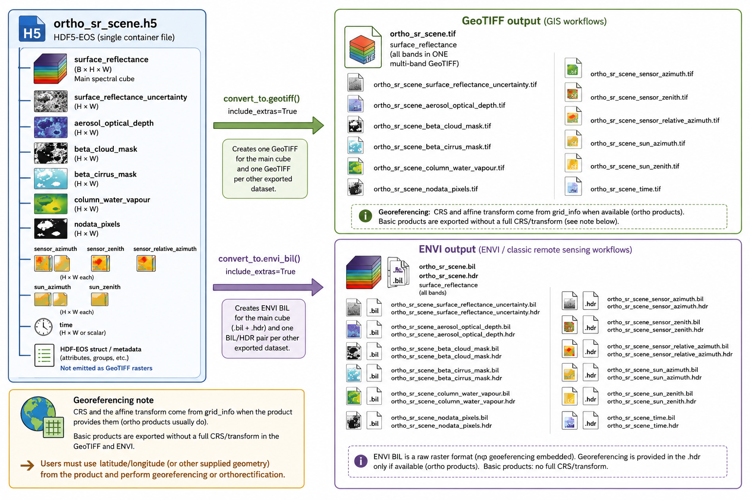
TanagerSpec bridges this gap using the .convert_to namespace. Calling tanager_ortho_sr.convert_to.geotiff() or tanager_ortho_sr.convert_to.envi_bil() automatically unpacks the internal HDF5 structure and routes the datasets into standalone files.

Comparing Export Formats¶

Method	Primary Output	Ancillary Layers (include_extras=True)
.convert_to.geotiff()	A single multi-band GeoTIFF containing the complete stacked surface_reflectance data cube.	Each extra layer (masks, optical depth, sensor angles) is written as its own individual GeoTIFF alongside the main cube.
.convert_to.envi_bil()	A binary .bil data file paired with a plain-text .hdr header file containing the main cube's band definitions.	Follows the same split logic: each companion dataset receives its own separate .bil and .hdr pair.

Later in this lesson, we also cover .convert_to.xarray(), which builds an in-memory xarray.Dataset instead of writing raster files to disk. That path is suited to Python-centric workflows and NetCDF export.

How Georeferencing is Handled¶

When exporting, TanagerSpec automatically checks the spatial metadata available in your source product to determine how to format the output headers:

• Ortho Products (ortho_sr): Because these scenes are fully orthorectified, TanagerSpec extracts the Coordinate Reference System (CRS) and affine transform matrix by parsing the metadata embedded in HDF5-EOS. These are seamlessly written into the exported GeoTIFF tags or ENVI header files, ensuring your files are positioned correctly in real-world coordinates as soon as they're loaded into GIS software.
• Basic Products (basic_sr): Basic scenes retain raw sensor geometry and do not include projected map coordinates. Consequently, exported GeoTIFFs and ENVI files will not contain a full CRS or transform matrix. If you export a basic product, you will need to utilize the separate latitude and longitude arrays supplied within the raw product to manually georeference or orthorectify the imagery using advanced GIS tools.

Visualizing the Export Output Mapping¶

To understand exactly what happens on your disk when you run an export with extra layers included, review the mapping hierarchy below. A single input HDF5 container splits cleanly into dedicated asset files:

Note

The exact same structural pattern applies. The primary cube becomes ortho_sr_scene.bil + .hdr, and each extra layer outputs as ortho_sr_scene_<layer_name>.bil + .hdr.

Executing the GeoTIFF Export¶

Let's start by exporting our scene to GeoTIFF. By setting include_extras=True, we instruct the converter to output not only the primary 426-band surface reflectance stack, but also standalone GeoTIFF rasters for our companion datasets (like cloud masks and sensor angles).

We will use the output_path parameter to route all these generated files cleanly into a dedicated geotiff sub-folder inside our main exports directory.

In [ ]:

# Create a dedicated sub-folder for GeoTIFF outputs to prevent file clutter
geotiff_out_dir = OUTPUT_DIR / "geotiff"
geotiff_out_dir.mkdir(exist_ok=True)

# Define the base name for the exported files
geotiff_base_path = geotiff_out_dir / "ortho_srsf_scene"

# Execute the GeoTIFF conversion
tanager_ortho_sr.convert_to.geotiff(
    output_path=geotiff_base_path,  # Base path and prefix for generated files
    include_extras=True             # True: export main cube + companion layers
)

print(f"GeoTIFF export complete! Check the folder: {geotiff_out_dir}")

# Create a dedicated sub-folder for GeoTIFF outputs to prevent file clutter geotiff_out_dir = OUTPUT_DIR / "geotiff" geotiff_out_dir.mkdir(exist_ok=True) # Define the base name for the exported files geotiff_base_path = geotiff_out_dir / "ortho_srsf_scene" # Execute the GeoTIFF conversion tanager_ortho_sr.convert_to.geotiff( output_path=geotiff_base_path, # Base path and prefix for generated files include_extras=True # True: export main cube + companion layers ) print(f"GeoTIFF export complete! Check the folder: {geotiff_out_dir}")

Executing the ENVI-BIL Export¶

Next, let's export the exact same raw data into the ENVI-BIL format. This format is highly favored by remote sensing scientists because binary files paired with readable .hdr text files load instantly into software like ENVI.

Just as before, setting include_extras=True will generate separate .bil and .hdr file pairs for every ancillary layer. To keep our workspace perfectly organized, we will direct these outputs into their own dedicated envi folder.

In [ ]:

# Create a dedicated sub-folder for ENVI outputs
envi_out_dir = OUTPUT_DIR / "envi"
envi_out_dir.mkdir(exist_ok=True)

# Define the base name for the exported files
envi_base_path = envi_out_dir / "ortho_sr_scene"

# Execute the ENVI-BIL conversion
tanager_ortho_sr.convert_to.envi_bil(
    output_path=envi_base_path,  # Base path and prefix for generated files
    include_extras=True          # True: export main cube + companion layers
)

print(f"ENVI-BIL export complete! Check the folder: {envi_out_dir}")

# Create a dedicated sub-folder for ENVI outputs envi_out_dir = OUTPUT_DIR / "envi" envi_out_dir.mkdir(exist_ok=True) # Define the base name for the exported files envi_base_path = envi_out_dir / "ortho_sr_scene" # Execute the ENVI-BIL conversion tanager_ortho_sr.convert_to.envi_bil( output_path=envi_base_path, # Base path and prefix for generated files include_extras=True # True: export main cube + companion layers ) print(f"ENVI-BIL export complete! Check the folder: {envi_out_dir}")

In-Memory xarray Conversion with .convert_to.xarray()¶

So far we have written scenes out as standalone raster files on disk. If your workflow stays inside Python, you can instead convert the current in-memory scene into an xarray.Dataset using .convert_to.xarray().

The returned Dataset includes:

• The hyperspectral cube as a DataArray named cube with dimensions (band, y, x)
• Coordinates band, y, and x (map coordinates for ortho products when grid metadata is available)
• Band metadata coordinates when present: wavelength, fwhm, and good_bands
• 2D quality masks and companion rasters from the source file as separate (y, x) variables
• Scene and geospatial metadata in Dataset .attrs (product_type, source_path, crs_wkt, epsg, transform, etc.)

Set include_secondary_cubes=True to also attach additional 3D layers whose shape matches the main cube (for example, surface_reflectance_uncertainty). This is analogous to exporting ancillary layers with include_extras=True on the disk converters, but limited to same-shape 3D datasets.

Once you have a Dataset, you can use standard xarray, Dask, and rioxarray workflows for analysis, lazy loading, and georeferenced I/O.

In [ ]:

# Convert the CURRENT in-memory scene to an xarray Dataset (nothing is written to disk).
# Because it captures the cube as it sits in memory, any preprocessing/denoising is reflected here.

ds = tanager_ortho_sr.convert_to.xarray(
    include_secondary_cubes=False,  # True also adds same-shape 3D layers, e.g. surface_reflectance_uncertainty
)

# Convert the CURRENT in-memory scene to an xarray Dataset (nothing is written to disk). # Because it captures the cube as it sits in memory, any preprocessing/denoising is reflected here. ds = tanager_ortho_sr.convert_to.xarray( include_secondary_cubes=False, # True also adds same-shape 3D layers, e.g. surface_reflectance_uncertainty )

In [ ]:

ds

ds

Exporting the Dataset to NetCDF¶

TanagerSpec does not provide a dedicated NetCDF writer. Because .convert_to.xarray() already assembles the scene as a standard xarray.Dataset, you can persist it with xarray's built-in Dataset.to_netcdf() method.

NetCDF is a common scientific interchange format and works well for sharing preprocessed cubes between Python tools. Because you are writing from the in-memory Dataset, the exported file reflects your current scene state—not the raw downloaded HDF5 baseline.

We will save the file into our timestamped exports directory alongside the GeoTIFF and ENVI outputs.

Note

Full ortho surface-reflectance scenes are large (426 bands). NetCDF export may take noticeable time and disk space. For exploratory work, consider subsetting or exporting a band slice first.

In [ ]:

# Replace -9999 values in the 'cube' DataArray with NaN, then plot band 100
ds_nan = ds.copy()

ds_nan["cube"] = ds_nan["cube"].where(ds_nan["cube"] != -9999, np.nan)

ds_nan.cube.sel(band=100).plot()

# Replace -9999 values in the 'cube' DataArray with NaN, then plot band 100 ds_nan = ds.copy() ds_nan["cube"] = ds_nan["cube"].where(ds_nan["cube"] != -9999, np.nan) ds_nan.cube.sel(band=100).plot()

In [ ]:

# Create a dedicated sub-folder for NetCDF outputs
netcdf_out_dir = OUTPUT_DIR / "netcdf"
netcdf_out_dir.mkdir(exist_ok=True)

# Define the output file path
netcdf_path = netcdf_out_dir / "ortho_sr_scene.nc"

# Save the xarray Dataset as a NetCDF file
ds.to_netcdf(netcdf_path)

print(f"NetCDF export complete! Check the folder: {netcdf_out_dir}")

# Create a dedicated sub-folder for NetCDF outputs netcdf_out_dir = OUTPUT_DIR / "netcdf" netcdf_out_dir.mkdir(exist_ok=True) # Define the output file path netcdf_path = netcdf_out_dir / "ortho_sr_scene.nc" # Save the xarray Dataset as a NetCDF file ds.to_netcdf(netcdf_path) print(f"NetCDF export complete! Check the folder: {netcdf_out_dir}")

What's Next?¶

Congratulations! You have successfully bridged the gap between raw Tanager hyperspectral container and standard Geographic Information System (GIS) workflows.

Whether you prefer to analyze your data directly in Python, as an xarray Dataset or NetCDF file, or export raw baselines to external GIS software, you now have complete control over your data management pipeline.

In the next lesson, we will jump back into our active Python workflow to explore Visualization. You will learn how to bring your preprocessed hyperspectral cubes to life by rendering true and false-color image composites and plotting rich spectral signatures directly inside your notebook.

See you in the next lesson!