
Welcome to Lesson 1 of Module 4 — Part 1. This part covers the conceptual and theoretical foundations of narrow-band spectral indices. You will learn why spectral indices are needed, how NDVI and EVI were developed and what their limitations are, how hyperspectral data enables more precise narrow-band analysis with Tanager-1, and which indices will be used in the hands-on Part 2. In Part 2 of this lesson, you will put these concepts into practice by computing all indices from real Tanager-1 scenes.
In this lesson, we are extending our understanding from Lesson 4 of Module 2, in which we delved deeper into spectral indices.
The main advantage of hyperspectral data when using spectral indices is that having many narrow, contiguous bands allow us to position wavelengths much more precisely around key absorption features and sensitive regions of the spectrum, such as the red edge. As a result, hyperspectral vegetation indices can be designed and tuned for many more specific properties including chlorophyll, water content, biomass, leaf area index (LAI), and other biophysical or biochemical characteristics.
Figure 1 illustrates this idea by comparing the continuous hyperspectral signature from Tanager-1 with the broader multispectral sampling of Sentinel-2. While Sentinel-2 captures reflectance in selected broad bands, Tanager-1 preserves the detailed shape of the spectrum across contiguous wavelengths. This added spectral detail allows hyperspectral data to support more precise and specialized index construction.
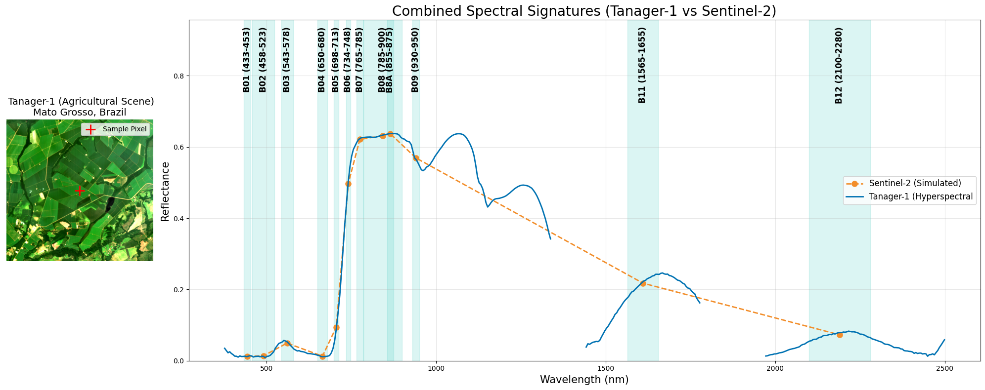
Figure 1:Comparison of a hyperspectral Tanager-1 spectral signature and a simulated multispectral Sentinel-2 spectral response. The hyperspectral curve preserves narrow, contiguous spectral detail, whereas the multispectral response samples only a limited number of broader bands.
For a broader perspective on how spectral band design affects remote-sensing applications, see NASA’s Spectral Bands and Applications page for Landsat. It shows how Landsat missions have progressively added and refined spectral bands since 1972, and how narrower visible and near-infrared bands in later sensors improved vegetation measurements and supported more specialized applications. Improvements in spectral band placement and spectral resolution for missions directly influence the kinds of analyses and indices we can develop.
Why Do We Need Spectral Indices?
Before we take advantage of hyperspectral data and calculate narrow-band spectral indices, we first need to understand why spectral indices are important and how they were developed.
In remote sensing, we usually do not rely on a single band alone. A single band can show brightness differences, but by itself it often does not tell us enough about the physical properties of the surface. Different materials may look similar in one band and very different in another. That is why combining information from multiple bands is so powerful: it helps us distinguish surface types and infer properties such as vegetation vigor, moisture, and stress.
Imagine that a sensor gives you only a red band image. Some areas may appear dark and others bright, but it is still difficult to know why. A dark response in the red band could be caused by vegetation, shadow, water, or another low-reflectance surface. Now imagine that the same sensor also gives you a near-infrared (NIR) band image of the same area. Suddenly, the pattern becomes much more informative. Vegetated fields that are dark in red often appear bright in NIR, and this contrast helps us distinguish them from other surfaces. In other words, the value of multispectral data is not simply that we have more images, but that each band captures a different part of how the surface interacts with light of varying wavelengths, as shown in Figure 2.
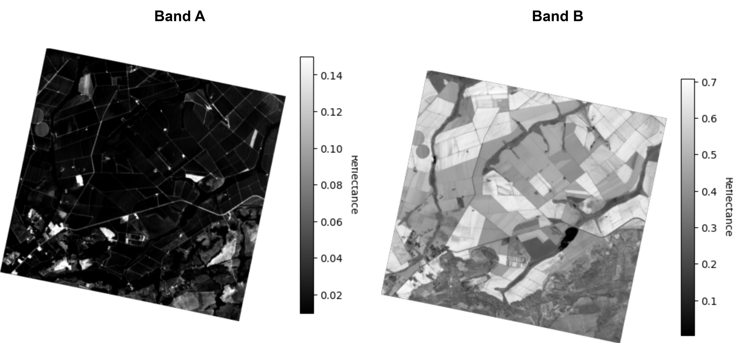
Figure 2:Band A (Red) and Band B (NIR)
Healthy vegetation is characterized by low reflectance in the red wavelengths and high reflectance in the near-infrared (NIR). Red light is strongly absorbed because of chlorophyll. These pigments absorb visible radiation for photosynthesis, particularly in the blue and red portions of the spectrum. By contrast, NIR radiation is only weakly absorbed by leaf biochemical constituents and is therefore largely scattered by the leaf’s internal structure and throughout the plant canopy as illustrated in Figure 3. This contrast between strong red absorption and high NIR reflectance is one of the most important spectral features used to identify and assess healthy green vegetation in remote sensing (Ustin & Jacquemoud, 2020Grondelle & Boeker, 2017). In unhealthy, senescent, or structurally damaged vegetation, this contrast weakens because stress reduces chlorophyll content and disrupts the mesophyll structure and intercellular air spaces, leading to higher red reflectance and lower NIR reflectance.
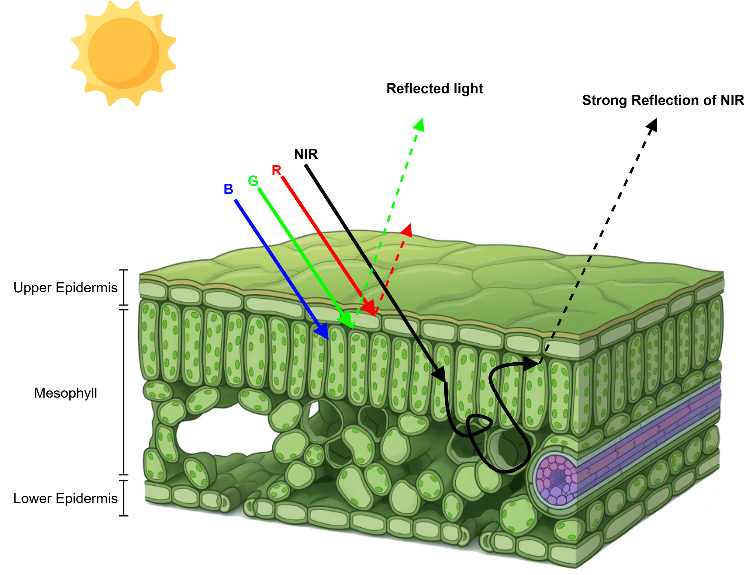
When vegetation becomes sparse, stressed, or unhealthy, the contrast between red and NIR reflectance decreases. Researchers recognized that this spectral difference could be used to monitor vegetation condition over large areas, leading to the development of vegetation indices (NASA Science).
Vegetation Index - NDVI
A vegetation index is designed to combine information from two or more spectral bands into a single value that is especially sensitive to vegetation while being less sensitive to irrelevant variation such as overall scene brightness. One of the earliest and most influential of these indices is the Normalized Difference Vegetation Index (NDVI). The normalized-difference approach was proposed in multispectral remote sensing work in 1973 Rouse et al., 1974, and the vegetation-monitoring form of NDVI became widely adopted during the early ERTS/Landsat era. (NASA Technical Reports)
NDVI is based on a simple but powerful idea: if vegetation reflects more NIR than red, then the contrast between those two bands should be positive and large. Rather than using only the raw difference, researchers used a normalized difference so that the index would be less sensitive to overall illumination and brightness:
: The reflectance of the surface in the Near-Infrared spectrum.
: The reflectance of the surface in the visible Red spectrum.
This concept is illustrated in Figure 4:
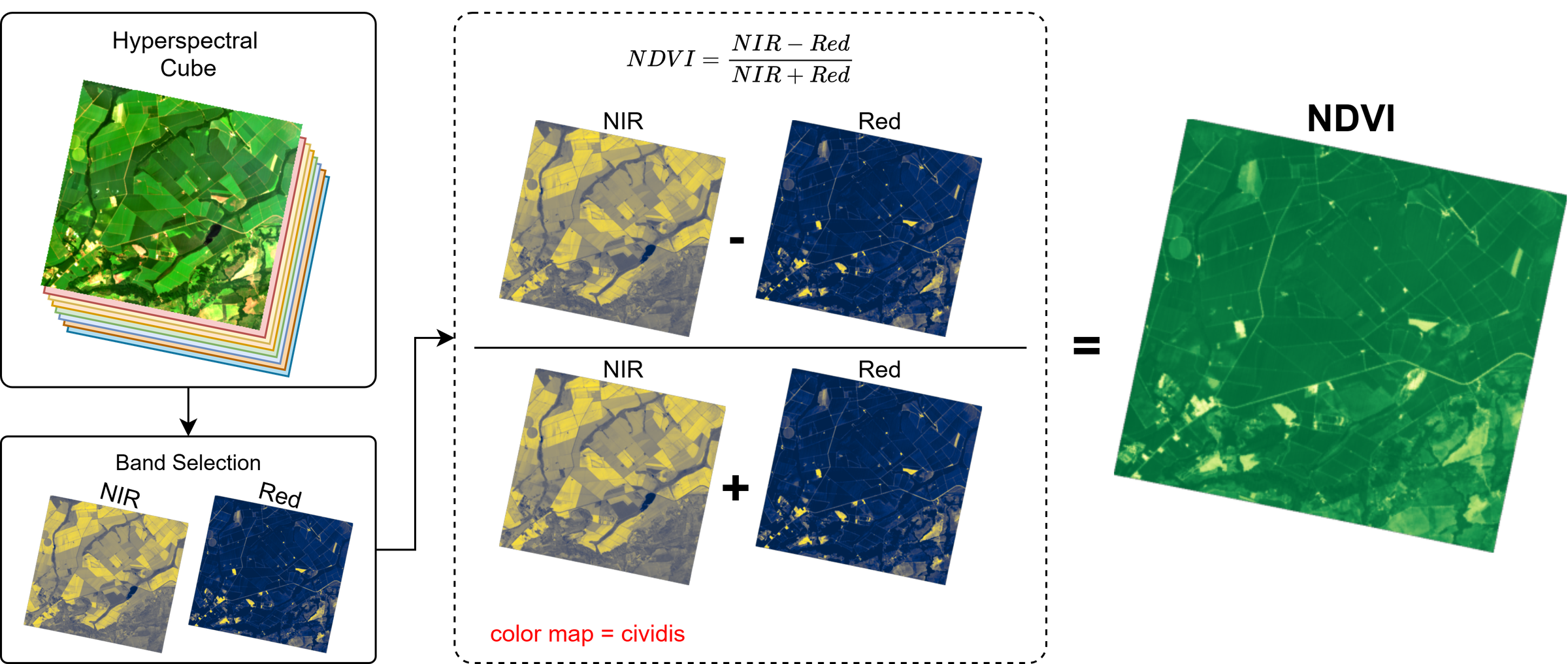
Figure 4:NDVI Calculation
In the classic multispectral case, NDVI uses a red band and a near-infrared band. In hyperspectral applications, the same concept can be implemented with narrow bands centered near the red absorption region and the NIR plateau. Common wavelength choices include approximately 680 nm (red) and 860 nm (NIR), though specific band selection may vary depending on sensor characteristics and application requirements. The result is a dimensionless index that typically ranges from -1 to +1. Higher values generally indicate greener and healthier vegetation, values near zero often correspond to bare soil or sparse cover, and negative values are most commonly associated with water, and can also indicate snow or clouds. ([NASA Science][1])
NDVI has been used extensively for monitoring vegetation condition, seasonal phenology, drought impacts, land-cover patterns, and broad changes in ecosystem productivity(NASA Technical Reports). However, NDVI also has important limitations. It tends to saturate in dense vegetation, meaning that once biomass becomes very high, further increases in vegetation do not produce equally large changes in NDVI Gitelson, 2004. It is also affected by atmospheric conditions and by background soil brightness, especially when vegetation cover is sparse. These limitations motivated the development of other indices such as EVI (Enhanced Vegetation Index) and SAVI (Soil-Adjusted Vegetation Index), which were designed to improve sensitivity in dense canopies and reduce atmospheric or soil-background effects. (USGS).
Enhanced Vegetation Index (EVI)
The Enhanced Vegetation Index (EVI) was designed as an improvement over NDVI for vegetation monitoring in complex canopy conditions. Both indices rely on the contrast between red absorption by chlorophyll and strong near-infrared reflectance from vegetation, but EVI extends this concept by incorporating the blue band together with correction terms for atmospheric aerosol effects and canopy-background adjustment. As a result, EVI reduces the influence of soil and atmospheric contamination and remains more sensitive than NDVI in high-biomass regions, where NDVI tends to saturate. For this reason, EVI is often better suited for distinguishing vegetation differences in dense canopies and for tracking structural vegetation properties beyond simple greenness (Huete et al., 2002).
EVI is designed to:
reduce saturation in high-biomass vegetation,
reduce the influence of canopy background and exposed soil,
reduce some atmospheric aerosol scattering effects by using the blue band.
The standard EVI formulation is:
where:
NIR = reflectance in the near-infrared band
R = reflectance in the red band
B = reflectance in the blue band
G = 2.5 — gain factor; scales the output so EVI values fall roughly in the same −1 to +1 range as NDVI, making them directly comparable.
L = 1 — canopy background adjustment; reduces the influence of exposed soil on the index when vegetation cover is sparse. A value of 1 is the standard for most land surfaces.
C₁ = 6, C₂ = 7.5 — aerosol resistance coefficients; use the blue band to partially correct for atmospheric aerosol scattering in the red band. These values were derived empirically from MODIS calibration data Huete et al., 2002 and should be treated as sensor-specific defaults.
While NDVI uses only red and NIR bands, EVI introduces additional terms that help stabilize the index when vegetation is dense or when background and atmospheric effects are important. Let’s plot the NDVI and EVI of an example from Tanager-1 open STAC agricultural scenes to compare the differences between these two indices (Figure 6).
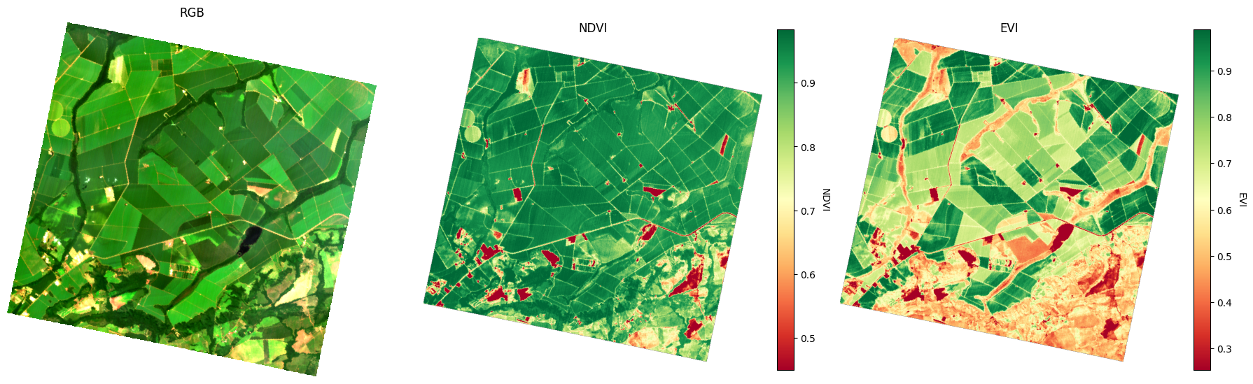
Figure 6:Comparison of RGB, NDVI, and EVI for a Tanager-1 scene in Brazil.
Interesting! As shown in Figure 6, most fields appear with very high NDVI values, indicating abundant vegetation cover. However, many of these fields look quite similar in NDVI, even though the RGB image suggests differences. In the EVI map, those same fields show significant variation. We can also see that field boundaries are more clearly separated in EVI, which means it is less affected by background noise and gives a cleaner view of vegetation condition. Let’s dive deeper into the distribution of both indices.
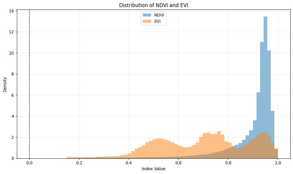
Figure 7:Distribution of NDVI and EVI values for the same Tanager-1 scene in Brazil.
As shown in Figure 7, the histogram highlights a clear difference between NDVI and EVI. The NDVI distribution is strongly left-skewed (negatively skewed) and tightly concentrated near the upper end of the scale, with most pixels clustered between 0.88 and 0.98. This indicates that the scene is dominated by vegetation, but it also shows that NDVI compresses many vegetated pixels into a narrow high-value range. As canopy density increases, NDVI becomes less able to distinguish moderate, high, and very high biomass.
In contrast, the EVI distribution is broader and appears multimodal, spanning roughly 0.2 to 1.0 with substantial density across the mid-to-high range. This wider spread shows that EVI preserves more internal variability within the scene. The shape of the distribution suggests multiple vegetation states or canopy conditions, which EVI separates more effectively than NDVI. In other words, NDVI shows that the scene is broadly very green, while EVI reveals meaningful differences within that vegetation. To make this saturation effect more explicit, we can now compare EVI and NDVI pixel by pixel in a scatterplot.
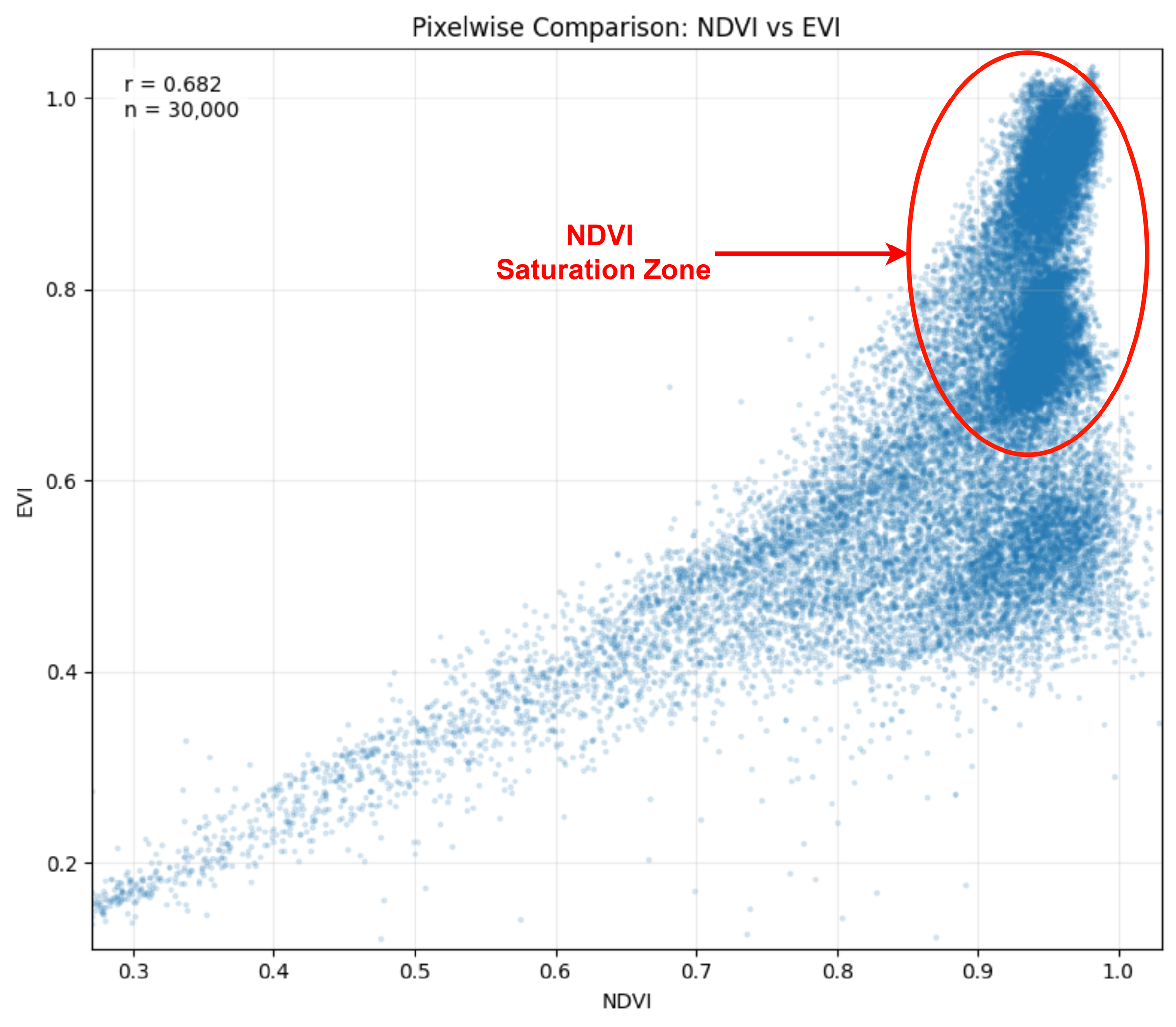
Figure 8:Pixelwise comparison of NDVI and EVI for the same Tanager-1 scene in Brazil.
As shown in Figure 8, the plot reveals great insights. At low to moderate vegetation levels, NDVI and EVI increase together, so the point cloud follows a clear upward trend. This means both indices respond similarly when vegetation cover is sparse to moderate. But once NDVI reaches high values, especially around 0.85 to 0.95 and above, the relationship changes. Instead of continuing to spread smoothly to the right, the points begin to form a nearly vertical cloud. That is the signature of saturation: many pixels have almost the same NDVI value, while their EVI values still vary substantially.
In other words, NDVI is no longer distinguishing well among these dense vegetation pixels. EVI, however, continues to separate those same pixels, giving different values for canopies that NDVI treats as nearly identical as you see in the red circled region. That wider vertical spread means EVI is retaining sensitivity to differences in canopy density, biomass, or vigor after NDVI has begun to level off. Taken together, the maps, histogram, and scatterplot tell the same story. NDVI is very effective for identifying vegetation, but in dense canopies it fails, while EVI reduces this problem and preserves more variability, making it especially useful for monitoring highly productive crops and dense vegetation.
From Multispectral Broadbands to Hyperspectral Narrowbands
So far, we have worked with NDVI and EVI, which were invented during the multispectral era. That means they rely on a small number of broad spectral bands, and although they are powerful, they only capture part of the information contained in the reflected signal. Hyperspectral data extends this capability by sampling the spectrum in many narrow and continuous bands. Instead of reducing vegetation to a single index, we can analyze the full spectral signature and link different parts of the spectrum to different plant traits. This opens the door to going beyond simple greenness mapping toward a more detailed assessment of vegetation properties such as chlorophyll, canopy density, water status, and biochemical composition.
Figure 9 shows a typical hyperspectral signature whose shape contains information about different plant properties, including pigments, canopy structure, leaf internal structure, water content, and dry matter constituents such as lignin and cellulose.
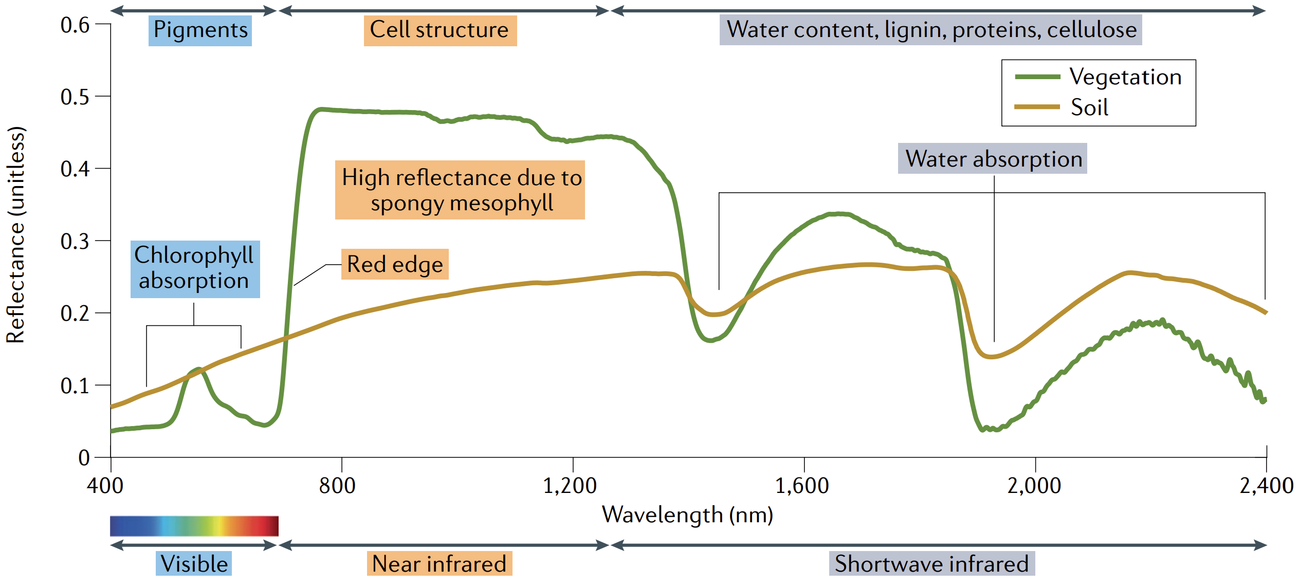
Figure 9:Typical spectral signature of healthy vegetation compared with soil. Credit: Zeng et al. (2022).
Vegetation indices tell us that vegetation is changing; hyperspectral signatures help us understand why it is changing.
Interpreting the Typical Vegetation Spectral Signature
A typical vegetation spectrum has a very characteristic shape, and each part of the spectral signature line is related to a different plant property.
Visible region (400–700 nm): pigments dominate
In the visible range, reflectance is mainly controlled by photosynthetic pigments, especially chlorophyll.
Reflectance is low in the blue and red parts of the spectrum because chlorophyll strongly absorbs light (energy) for photosynthesis.
Reflectance is relatively higher in the green region, which is why healthy vegetation appears green to our eyes.
Red edge (~680–750 nm): rapid transition
Around the boundary between red and near-infrared, the vegetation spectrum rises very sharply. This feature is called the red edge. The red edge occurs because the chlorophyll absorption decreases rapidly after the red wavelengths, while internal leaf scattering becomes dominant in the near-infrared. The position and steepness of the red edge are very informative and are often linked to vegetation status, chlorophyll content, and canopy condition.
Near-infrared (NIR, ~750–1300 nm): leaf and canopy structure dominate
In the near-infrared, healthy vegetation has high reflectance. This is not because of pigments, but mainly because of the internal structure of the leaf, especially scattering within the spongy mesophyll, and also because of canopy architecture. This is why vegetation indices based on red and NIR work so well: vegetation strongly absorbs red light but strongly reflects NIR light. This region is often related to:
leaf internal structure,
canopy density,
biomass,
and often LAI, especially when comparing fields with different canopy development.
Shortwave infrared (SWIR, ~1300–2500 nm): water and dry matter dominate
In the shortwave infrared, reflectance is influenced by leaf water content and biochemical constituents such as: lignin, cellulose, proteins, and other dry matter components. The deep absorption features near about 1400 nm and 1900 nm are mainly due to water absorption (back to lesson 4 module 2). Other parts of the SWIR are affected by biochemical composition and tissue properties. This means SWIR is especially useful when we want to study:
water stress,
moisture content,
dry matter,
and plant composition.
Now, let’s connect EVI and hyperspectral data to see if fields with different EVI values have different spectral signatures, especially in the red-edge and near-infrared regions. We can test this by comparing spectral signatures from fields with varying EVI levels within the same Tanager-1 scene from Brazil.
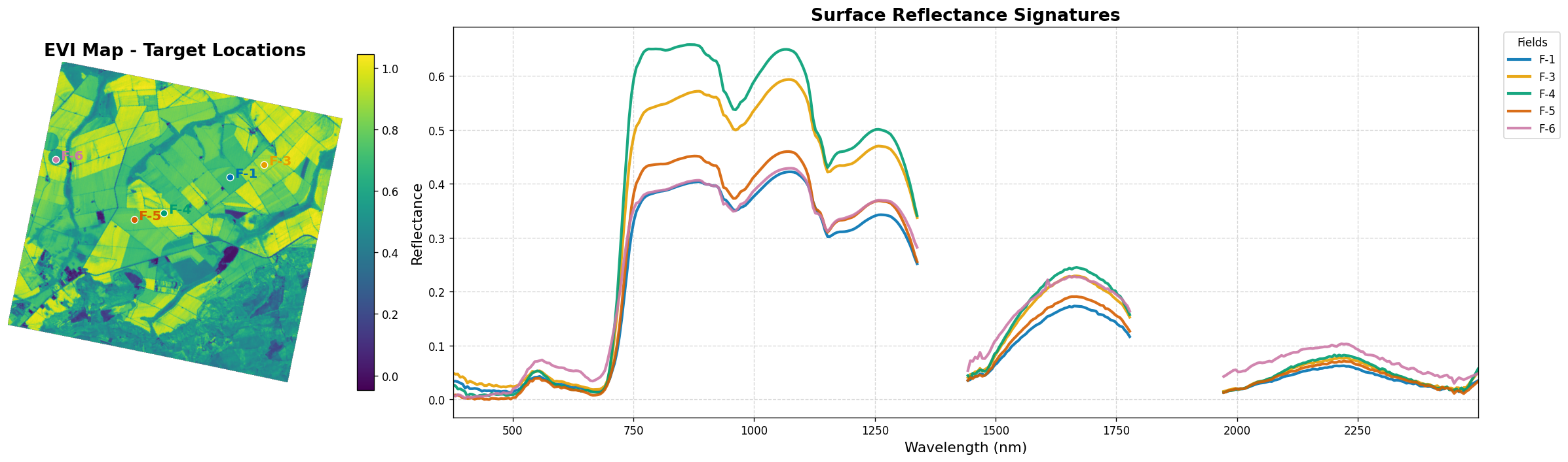
Figure 10:Spectral signatures from various fields exhibiting different EVI values
As shown in Figure 10, these spectra show that the EVI differences are physically meaningful. The fields with higher EVI also tend to have a steeper red edge and a higher NIR reflectance, which is what we expect from denser canopies and higher biomass. So EVI is not just producing arbitrary contrast; it is tracking real vegetation structure. But the SWIR also shows differences between fields, which tells us that hyperspectral data adds information beyond EVI, especially about water and biochemical properties.
The field spectra suggest that higher EVI corresponds to stronger canopy development, especially through higher NIR reflectance. To test whether this interpretation is physically consistent with canopy radiative transfer theory, we can compare it with simulations from PROSPECT-D and 4SAIL, where LAI is varied explicitly and the resulting spectral signature is modeled.
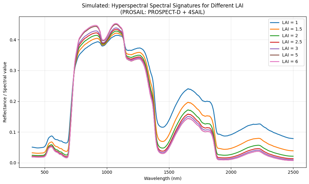
Figure 11:Simulated canopy reflectance for increasing LAI using the PROSAIL: PROSPECT-D + 4SAIL radiative transfer model.
To interpret hyperspectral signatures more confidently, we often use radiative transfer models. In this case, the PROSAIL model is used. It combines PROSPECT-D, which simulates how an individual leaf interacts with light based on its biochemical and structural properties, with 4SAIL, which simulates how a canopy of many leaves reflects light, taking into account canopy architecture and viewing geometry. This model is widely used to understand how vegetation properties such as Leaf Area Index (LAI) affect spectral reflectance.
This is important because it helps us answer a key question:
If EVI is really responding to biomass or canopy development, then should the spectral signature change in a predictable way when LAI increases?
As shown in Figure 11, the answer is yes. Increasing LAI produces a stronger red-edge/NIR response, which is consistent with the higher NIR reflectance observed in the higher-EVI fields. This supports the interpretation that EVI in this scene is tracking biomass- or canopy-density-related variation. Also, as LAI increases you can see reflectance decreases in the visible due to stronger pigment absorption.
From Multispectral Indices to Tanager-1 Narrow-Band Analysis
NDVI and EVI were developed in the multispectral era, when most satellite sensors provided only a small number of broad spectral bands. That is why they are so useful: they summarize vegetation condition efficiently using only a few wavelength regions, especially the red, blue, and near-infrared. But this is also their main limitation, because broad bands average over important absorption and scattering features that contain more specific information about plant condition.
This is where Tanager-1 becomes especially valuable. Tanager-1 captures approximately 426 narrow bands with roughly 5 nm spacing across a spectral range of 380–2500 nm at ~30 m spatial resolution. Instead of working with only a few broad multispectral bands, we can examine the full spectral shape of vegetation in much finer detail. That allows us to target narrow spectral features such as the red edge, chlorophyll-sensitive bands, and water-absorption regions in the SWIR.
So in the context of Tanager-1, this lesson naturally extends from NDVI and EVI to narrow-band vegetation analysis. NDVI and EVI tell us that vegetation differs, but Tanager-1 allows us to investigate why it differs by isolating spectral features related to chlorophyll, canopy structure, photosynthetic function, and water status.
The field of remote sensing spectral indices is vast. For this lesson, we will focus on two applications of remote sensing: vegetation and water bodies. Since vegetation is a widely studied topic, we will focus on a small and targeted set of indices: NDRE (Normalized Difference Red Edge), REP (Red Edge Position), PRI (Photochemical Reflectance Index) Gamon et al., 2012, and NDWI for vegetation water content Gao, 1996. Note that a different NDWI formulation McFeeters, 1996 will be used later for water body delineation.
Indices Used in This Lesson — Quick Reference
The table below summarises every index calculated in this lesson. Use it as a cheat sheet when interpreting results.
| Index | Full Name | Wavelengths Used | What It Measures | Typical Range |
|---|---|---|---|---|
| NDVI | Normalized Difference Vegetation Index | Red (~670 nm), NIR (~860 nm) | General vegetation greenness | −1 to +1 |
| EVI | Enhanced Vegetation Index | Blue (~475 nm), Red (~670 nm), NIR (~800 nm) | Greenness with atmospheric/soil correction | −1 to +1 |
| REP | Red Edge Position | 680, 700, 740, 780 nm | Chlorophyll via red-edge wavelength shift | 700–740 nm |
| NDRE | Normalized Difference Red Edge | Red edge (~740 nm), NIR (~800 nm) | Chlorophyll amplitude; less saturation than NDVI | −1 to +1 |
| PRI | Photochemical Reflectance Index | 531 nm, 570 nm | Xanthophyll/carotenoid pigment ratio | −0.2 to +0.1 |
| NDWI_veg | NDWI — Vegetation Water (Gao 1996) | NIR (~860 nm), SWIR (~1240 nm) | Canopy liquid water content | −1 to +1 |
| NDWI_water | NDWI — Open Water (McFeeters 1996) | Green (~560 nm), NIR (~842 nm) | Water body delineation | −1 to +1 |
| NDCI | Normalized Difference Chlorophyll Index | Red edge (~705 nm), Red (~665 nm) | Chlorophyll-a in water (algal bloom proxy) | −1 to +1 |
What’s Next
This lesson has introduced the conceptual foundations of narrow-band spectral indices: the motivation behind spectral indices, the evolution from NDVI to EVI, the structure of a typical vegetation spectral signature, and the set of indices — REP, NDRE, PRI, NDWI, and NDCI — that Tanager-1’s ~5 nm hyperspectral bands make possible.
In Part 2, you will put these ideas into practice. You will load two real Tanager-1 scenes, compute each index using helper functions, and interpret the spatial patterns across an agricultural landscape in Brazil and a water body scene in South Korea.
- Ustin, S. L., & Jacquemoud, S. (2020). How the optical properties of leaves modify the absorption and scattering of energy and enhance leaf functionality. In S. Liang (Ed.), Remote Sensing of Plant Biodiversity (pp. 349–384). Springer. 10.1007/978-3-030-33157-3
- van Grondelle, R., & Boeker, E. (2017). Limits on Natural Photosynthesis. The Journal of Physical Chemistry B, 121(30), 7229–7234. 10.1021/acs.jpcb.7b03024
- Rouse, J. W., Haas, R. H., Schell, J. A., & Deering, D. W. (1974). Monitoring Vegetation Systems in the Great Plains with ERTS (Techreport NASA SP-351). NASA. https://ntrs.nasa.gov/citations/19740022614
- Gitelson, A. A. (2004). Wide dynamic range vegetation index for remote quantification of biophysical characteristics of vegetation. Journal of Plant Physiology, 161(2), 165–173.
- Huete, A., Didan, K., Miura, T., Rodriguez, E. P., Gao, X., & Ferreira, L. G. (2002). Overview of the radiometric and biophysical performance of the MODIS vegetation indices. Remote Sensing of Environment, 83(1–2), 195–213. 10.1016/S0034-4257(02)00096-2
- Huete, A. R. (1988). A soil-adjusted vegetation index (SAVI). Remote Sensing of Environment, 25(3), 295–309.
- Jiang, Z., Huete, A. R., Didan, K., & Miura, T. (2008). Development of a two-band enhanced vegetation index without a blue band. Remote Sensing of Environment, 112(10), 3833–3845.
- Zeng, Y., Hao, D., Huete, A., & others. (2022). Optical vegetation indices for monitoring terrestrial ecosystems globally. Nature Reviews Earth & Environment, 3, 477–493. 10.1038/s43017-022-00298-5
- Gamon, J. A., Peñuelas, J., & Field, C. B. (2012). A narrow-waveband spectral index that tracks diurnal changes in photosynthetic efficiency. New Phytologist. 10.1111/j.1469-8137.2011.03791.x
- Gao, B.-C. (1996). NDWI—A normalized difference water index for remote sensing of vegetation liquid water from space. Remote Sensing of Environment, 58(3), 257–266.
- McFeeters, S. K. (1996). The use of the Normalized Difference Water Index (NDWI) in the delineation of open water features. International Journal of Remote Sensing, 17(7), 1425–1432. 10.1080/01431169608948714