
Welcome to the last lesson in the Analysis and Applications module.
In the previous lessons, we focused on managing the high dimensionality of hyperspectral data using Principal Component Analysis (PCA) to reduce dimensionality, remove noise, and reconstruct cleaner hyperspectral cubes.
In this lesson, we move from dimensionality reduction to clustering, an unsupervised machine learning technique that groups similar pixels together based on their spectral signatures—without requiring predefined class labels.
Why is clustering useful for hyperspectral data?
In many real-world applications, we don’t know in advance what materials or land-cover types are present in an image. Clustering allows us to explore the data and discover natural groupings that may represent distinct surface types, such as different vegetation conditions, soil types, water bodies, or urban materials.
The key question clustering helps us answer is:
Do the pixels in this hyperspectral image naturally form meaningful groups based on their spectral signatures?
What you’ll learn in this lesson:
How to prepare hyperspectral data for clustering
How k-means clustering groups pixels based on spectral similarity
How to interpret clustering results using spatial maps and mean spectral signatures
How to compare clustering results from different input features (full cube, RGB, PCA components)
Hyperspectral Cube for This Lesson
We will continue using the same agricultural scene from the previous lesson near Campo Verde, Mato Grosso, Brazil. This scene is well-suited for clustering because it contains diverse land-cover types, including:
Agricultural fields with varying crop conditions
Water bodies
Roads and bare soil
Different vegetation types
This diversity makes it a useful test case for exploring whether k-means clustering can identify and separate distinct spectral groups based on surface characteristics.
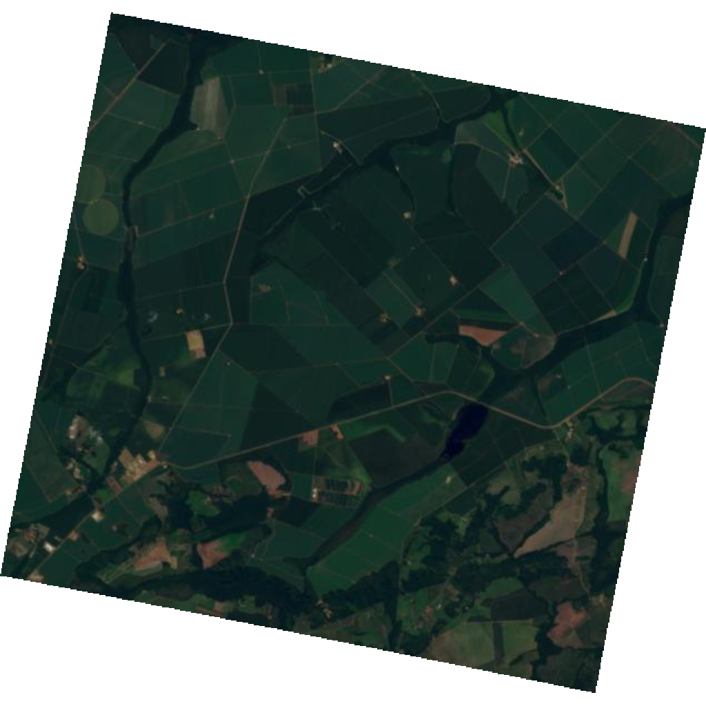
Scene: Tanager-1 scene near Campo Verde, Mato Grosso, Brazil.
Imports and global settings
The next cell imports all packages used in the lesson and keeps global settings in one place.
🧰 Your Toolkit so far
The reference solution for your full toolkit through Module 4 · Lesson 3 — loader,
band/RGB helpers, safe index math, flatten_cube/run_pca, and the spectral-similarity
metrics. Keep it at the top and run it first. This capstone adds the final pieces:
select_wavelengths and the K-means workflow helpers.
# ==================
# 🧰 YOUR TOOLKIT  (reference solution so far — through Module 4 · Lesson 3)
# ==================

# Essential imports
import h5py
import numpy as np
import matplotlib.pyplot as plt
import pandas as pd
from sklearn.cluster import KMeans
from sklearn.decomposition import PCA
from sklearn.preprocessing import StandardScaler
from sklearn.metrics import adjusted_rand_score, normalized_mutual_info_score

# Reproducibility for PCA / clustering
RANDOM_STATE = 31

# ---- setup -------------------------------------------------------------

def download_tanager_data(url, file_path):
    import os
    import urllib.request

    def _progress(count, block_size, total_size):
        mb_done = count * block_size / 1_000_000
        mb_total = total_size / 1_000_000
        print(f"\rDownloading... {mb_done:.1f} / {mb_total:.1f} MB", end="", flush=True)

    if not os.path.exists(file_path):
        urllib.request.urlretrieve(url, file_path, reporthook=_progress)
        print(f"\nDownload complete: {file_path}")
    else:
        print(f"File already exists, skipping download: {file_path}")
    return file_path

# ---- io ----------------------------------------------------------------

def load_hdf5(
    file_path,
    data_path='HDFEOS/GRIDS/HYP/Data Fields/surface_reflectance',
    nodata_path='HDFEOS/GRIDS/HYP/Data Fields/nodata_pixels',
    clean=True,
    band=None
    ):

    with h5py.File(file_path, 'r') as f:
        dset = f[data_path]
        # select all or a single band
        if band is None:
            data = dset[:].astype(np.float32)
        else:
            data = dset[band].astype(np.float32)
        attrs = dict(dset.attrs)

        wavelengths = np.asarray(attrs['wavelengths'], dtype=np.float32)
        good = np.asarray(attrs['good_wavelengths'], dtype=bool)
        no_data = f[nodata_path][:].astype(bool)

    if clean:
        if band is None:
            data = data[good]
            wavelengths = wavelengths[good]
            data[:, no_data] = np.nan
            good = good[good]
        else:
            # For a single band, check if it is good, else return all nan
            wavelengths = np.array([wavelengths[band]], dtype=np.float32)
            if not good[band]:
                data = np.full_like(data, np.nan)
            else:
                data[no_data] = np.nan
            good = np.array([good[band]], dtype=bool)

    attrs['wavelengths'] = wavelengths
    attrs['good_wavelengths'] = good

    return data, attrs, no_data

# ---- bands -------------------------------------------------------------

def nearest_band(wavelengths, target_nm):
    return int(np.argmin(np.abs(np.asarray(wavelengths) - target_nm)))

# ---- transform ---------------------------------------------------------

def flatten_cube(cube, no_data=None):

    bands, rows, cols = cube.shape
    X = cube.reshape(bands, rows * cols).T
    valid_mask = np.isfinite(X).all(axis=1)
    if no_data is not None:
        valid_mask &= ~no_data.ravel()
    X_valid = X[valid_mask]
    return X, X_valid, valid_mask

def run_pca(X, n_components=10, scale=False, random_state=RANDOM_STATE):
    scaler = None
    X_input = X
    if scale:
        scaler = StandardScaler()
        X_input = scaler.fit_transform(X)
    pca_model = PCA(n_components=n_components, random_state=random_state)
    X_pca = pca_model.fit_transform(X_input)
    return X_pca, pca_model, scaler


# ---- visualization ----------------------------------------------------

def make_rgb(cube, wavelengths, r_nm=680, g_nm=550, b_nm=470,
             percentile_low=2, percentile_high=98, reference_cube=None):
    """Create a display RGB using per-channel percentile stretching.

    If `reference_cube` is provided, display limits are computed from both cubes
    so before/after RGB images use the same stretch.
    """
    r = nearest_band(wavelengths, r_nm)
    g = nearest_band(wavelengths, g_nm)
    b = nearest_band(wavelengths, b_nm)
    band_indices = (r, g, b)

    rgb = np.dstack([cube[idx] for idx in band_indices]).astype(np.float32)
    if reference_cube is None:
        stretch_rgb = rgb
    else:
        reference_rgb = np.dstack([reference_cube[idx] for idx in band_indices]).astype(np.float32)
        stretch_rgb = np.concatenate([rgb, reference_rgb], axis=0)

    rgb_display = np.zeros_like(rgb, dtype=np.float32)
    for channel in range(3):
        p_low, p_high = np.nanpercentile(
            stretch_rgb[:, :, channel],
            (percentile_low, percentile_high)
        )
        if not np.isfinite(p_low) or not np.isfinite(p_high) or p_high <= p_low:
            continue
        rgb_display[:, :, channel] = (rgb[:, :, channel] - p_low) / (p_high - p_low)

    return np.clip(rgb_display, 0, 1)
# Download the Tanager-1 Ortho SR HDF5 file using the provided
# download_tanager_data helper (defined just above).
url = "https://storage.googleapis.com/open-cogs/planet-stac/tanager1-release2-core-imagery/ortho_sr_hdf5/20250501_143138_87_4001_ortho_sr_hdf5.h5"
file_path = "20250501_143138_87_4001_ortho_sr_hdf5.h5"
download_tanager_data(url, file_path)File already exists, skipping download: 20250501_143138_87_4001_ortho_sr_hdf5.h5
'20250501_143138_87_4001_ortho_sr_hdf5.h5'Unsupervised and Supervised Learning
Before introducing K-means, it is important to understand the difference between supervised learning and unsupervised learning.
In supervised learning, the dataset contains both the input data and the correct labels. For example, in hyperspectral image classification, each pixel may have spectral values from many bands, and each pixel may also have a label such as vegetation, soil, water, or urban area. The model learns from these labeled examples and then uses what it learned to classify new pixels.
In unsupervised learning, the dataset does not include labels. The algorithm only receives the input data, such as an array or table of pixel values, and tries to find patterns or groups by itself. This is useful when we have hyperspectral data but do not have reference labels telling us what each pixel represents.
In the second case, the algorithm does not know whether a pixel is vegetation, soil, water, or another material. It only sees the numerical values and tries to group pixels that are similar, as illustrated in Figure 1.
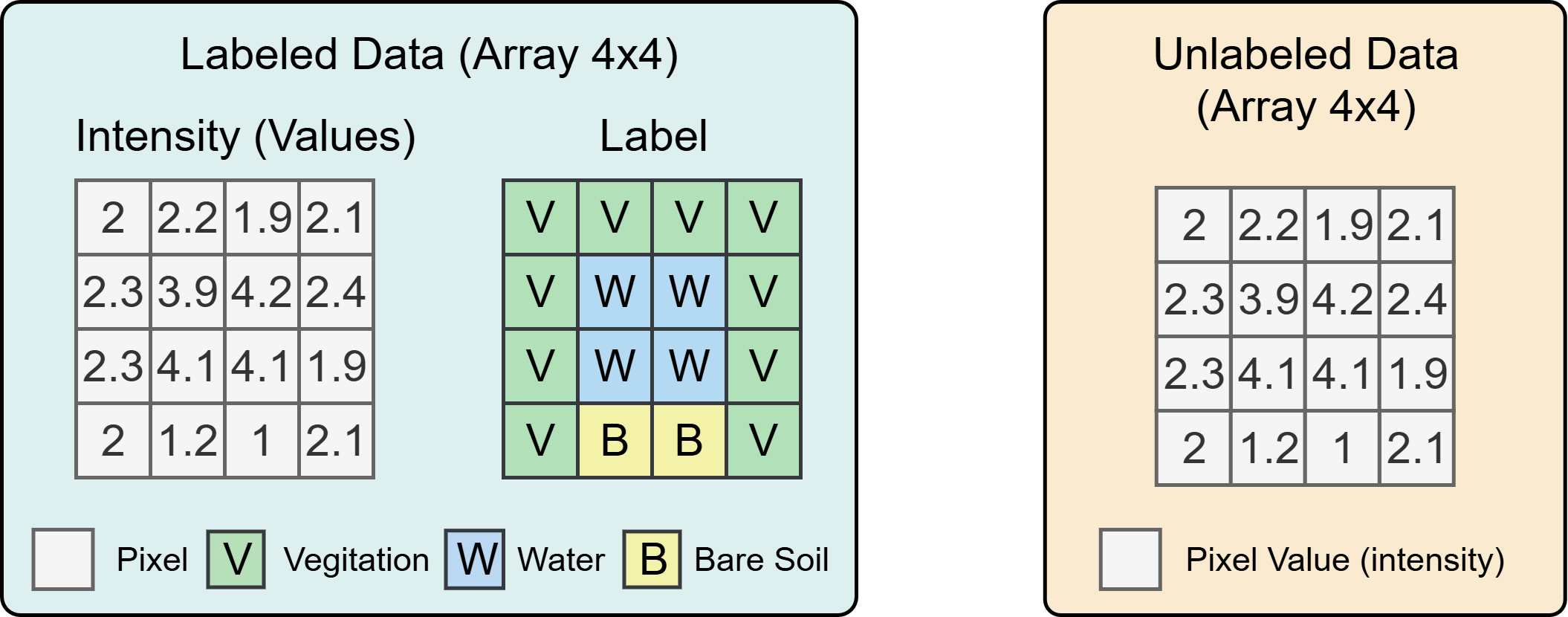
Figure 1:Labeled vs. unlabeled data structure for machine learning.
What is K-means?
K-means is an unsupervised clustering algorithm that groups pixels with similar spectral signatures together. The name tells you exactly what it does:
K = the number of clusters you want to create
Means = the algorithm finds the mean (average) spectral signature for each cluster
How does K-means work with hyperspectral data?
Each pixel in a hyperspectral image is represented by a spectral signature—a vector of reflectance values across hundreds of bands. For Tanager-1 data with 426 bands, each pixel is a 400+-dimensional vector.
K-means compares these vectors and groups pixels with similar spectral signatures into the same cluster. The resulting clusters often correspond to distinct materials or land-cover types, such as vegetation, soil, water, or different crop conditions.
The K-means Algorithm
K-means works by minimizing the variance within each cluster. It uses an iterative 5-step process:
1. Choose the number of clusters (K)
You must decide how many clusters to create. For example:
K = 3 might separate major classes found in the image like “Water,” “Vegetation,” and “Soil”
K = 10 might reveal finer distinctions like different crop types or soil moisture levels
2. Initialize cluster centroids
The algorithm randomly selects K starting points (centroids) from the data. Each centroid represents the “center” of a cluster.
3. Assign pixels to nearest centroid
Every pixel is assigned to the cluster whose centroid is closest, typically using Euclidean distance (the straight-line distance in high-dimensional space).
4. Update centroids
After all pixels are assigned, recalculate each centroid as the mean spectral signature of all pixels in that cluster.
5. Repeat until convergence
Steps 3 and 4 repeat until the centroids stop moving and cluster assignments stabilize, as shown in Figure 2.
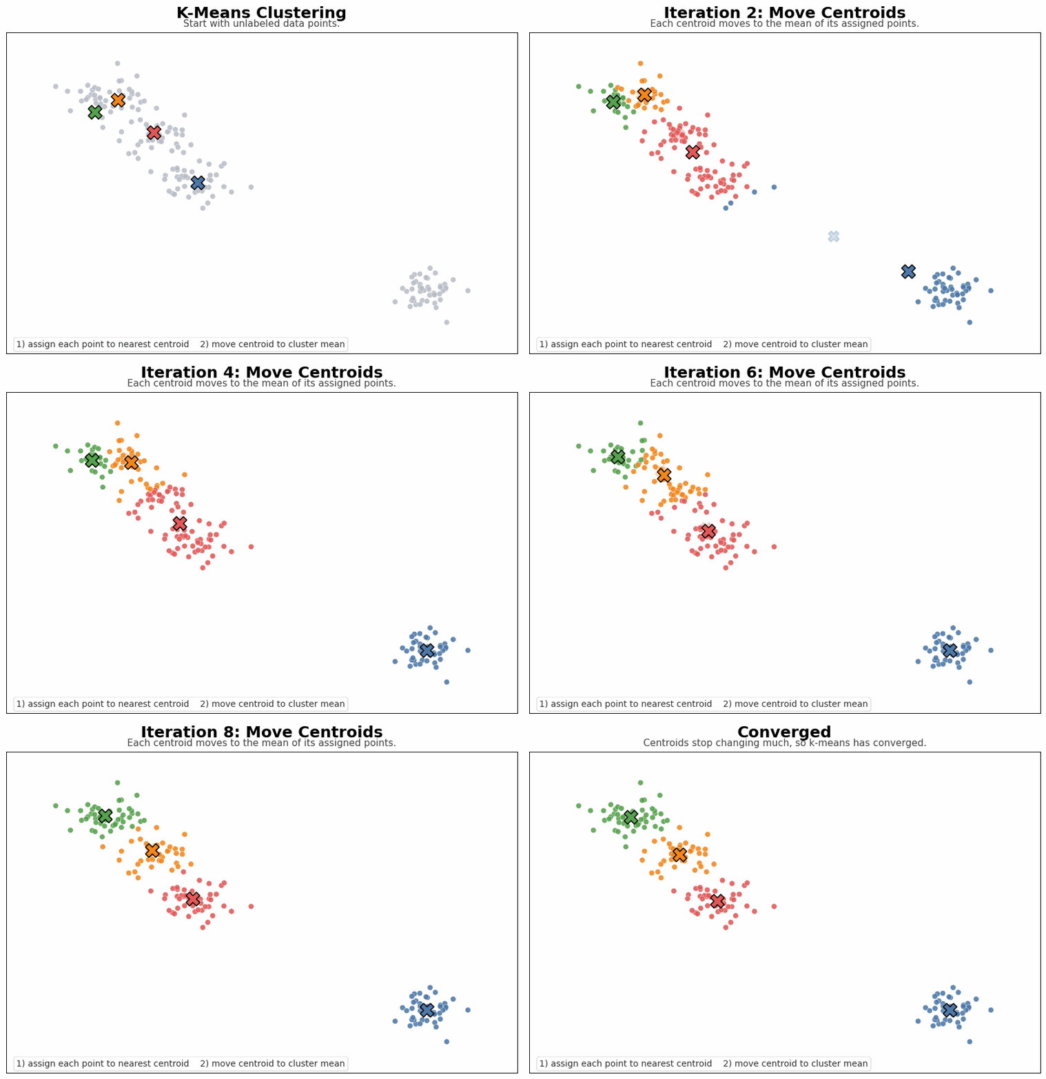
Figure 2:How K-means clustering works.
The algorithm starts with initial centroids, assigns each point to the nearest centroid, updates the centroid locations, and repeats until the clusters stabilize.
Mathematical objective:
K-means minimizes the Within-Cluster Sum of Squares (WCSS):
Where:
= total variance to minimize
= number of clusters
= a pixel’s spectral signature
= centroid of cluster
= squared distance between pixel and centroid
Now that we have established the foundation of K-means, it is time to move from theory to execution.
Building Your Final Toolkit Additions
This capstone adds the last pieces to your Toolkit: select_wavelengths (optional spectral
subsetting on top of the file’s good_wavelengths) and the K-means workflow helpers
(run_kmeans_clustering, labels_to_map, plot_kmeans_cluster_map, run_and_plot_kmeans,
plot_cluster_maps). Each is defined inline where it’s first used, and the complete
library is collected at the end of the lesson.
Preprocessing Considerations Before Clustering
Before applying K-means, we need to prepare the hyperspectral data carefully. The preprocessing choices we make will strongly influence the clustering results.
Key preprocessing decisions:
Which bands to include - Remove noisy or atmospheric absorption bands
Which pixels to mask - Exclude clouds, shadows, and no-data pixels
Whether to normalize - Raw reflectance vs. standardized values
Whether to reduce dimensionality - Use all bands vs. PCA components
Why does this matter for K-means?
K-means groups pixels based on Euclidean distance in feature space. This means:
Bands with larger values or variance have more influence on the clustering
In vegetation scenes, NIR bands (high reflectance) may dominate over visible bands (lower reflectance)
The clustering may emphasize brightness differences rather than spectral shape differences
For this lesson, we’ll start with as-retrieved reflectance values and compare results across different feature sets.
Lesson Approach
In this lesson, we’ll compare three clustering approaches:
Full hyperspectral cube - using all spectral bands directly
RGB bands only - using just three visible wavelengths
PCA components - using dimensionality-reduced features
By comparing these results, you’ll see how input feature selection affects clustering quality and learn to interpret cluster maps using both spatial patterns and spectral signatures.
Loading and Data Preparation
The original HDF5 file stores the hyperspectral cube as (bands, rows, columns).
Our load_tanager_hdf5 function automatically handles the initial preprocessing by dropping bad bands and setting no-data pixels to NaN, so we can proceed directly to preparing the data for K-means clustering.
cube, attrs, no_data = load_hdf5(file_path)

wavelengths = attrs['wavelengths']

bands, rows, cols = cube.shape

print(f"Cube shape: {cube.shape}  (bands, rows, cols)")
print(f"Wavelength range after good_wavelengths mask: {wavelengths.min():.1f}–{wavelengths.max():.1f} nm")
Cube shape: (368, 752, 784) (bands, rows, cols)
Wavelength range after good_wavelengths mask: 376.4–2499.0 nm
Preprocessing for K-means
We’ve already dropped bad bands and masked invalid pixels. The next step is to flatten the hyperspectral cube from 3D (bands, rows, cols) to 2D (pixels, bands) format, which both PCA and K-means require.
Optional: Additional band filtering
The next code cell allows you to filter specific wavelength ranges. For example, you could run K-means on only the visible, NIR, or SWIR portions of the spectrum.
Optional spectral subsetting: select_wavelengths
Your loader already drops the file’s flagged bad bands. Sometimes you also want to restrict
clustering to a wavelength range (e.g. visible-only, or excluding noisy water-vapour bands).
select_wavelengths returns a Boolean keep-mask you can apply to both the cube and the
wavelength array — it’s the last general helper we add to the Toolkit.
# Added to your Toolkit this lesson: a flexible wavelength keep-mask.
def select_wavelengths(wavelengths, min_nm=None, max_nm=None, exclude_ranges=None):
    """Return a Boolean mask for wavelengths to keep.

    Parameters
    ----------
    wavelengths : ndarray
        Array of wavelength values in nanometers.
    min_nm : float, optional
        Minimum wavelength to keep (inclusive).
    max_nm : float, optional
        Maximum wavelength to keep (inclusive).
    exclude_ranges : list of tuples, optional
        List of (low, high) wavelength ranges to exclude.

    Returns
    -------
    keep : ndarray, dtype=bool
        Boolean mask where True indicates wavelengths to keep.
    """
    keep = np.ones_like(wavelengths, dtype=bool)
    if min_nm is not None:
        keep &= wavelengths >= min_nm
    if max_nm is not None:
        keep &= wavelengths <= max_nm
    if exclude_ranges is not None:
        for low, high in exclude_ranges:
            keep &= ~((wavelengths >= low) & (wavelengths <= high))
    return keep
# Optional wavelength filtering after the file's built-in good_wavelengths mask.
# For example, you could later run the K-means analysis on only visible, NIR, or SWIR wavelengths.
# Set to True to apply additional wavelength filtering, False to use all good wavelengths
APPLY_EXTRA_WAVELENGTH_FILTER = True
MIN_WAVELENGTH_NM = 370
MAX_WAVELENGTH_NM = 2500
EXCLUDE_WAVELENGTH_RANGES = None # Example: [(1350, 1450), (1800, 1950)]
# Apply the wavelength filter based on the settings above
if APPLY_EXTRA_WAVELENGTH_FILTER:
keep = select_wavelengths(
wavelengths,
min_nm=MIN_WAVELENGTH_NM,
max_nm=MAX_WAVELENGTH_NM,
exclude_ranges=EXCLUDE_WAVELENGTH_RANGES,
)
else:
# Keep all wavelengths (no additional filtering)
keep = np.ones_like(wavelengths, dtype=bool)
# Create the filtered cube and wavelength array
cube_clean = cube[keep]
wavelengths_clean = wavelengths[keep]
bands_clean, rows_clean, cols_clean = cube_clean.shape
# Print summary of filtering results
print(f"Bands before extra filtering: {bands}")
print(f"Bands after extra filtering: {bands_clean}")
print(f"Clean wavelength range: {wavelengths_clean.min():.1f}–{wavelengths_clean.max():.1f} nm")Bands before extra filtering: 368
Bands after extra filtering: 368
Clean wavelength range: 376.4–2499.0 nm
The next cell flattens the cube from (bands, rows, columns) to (pixels, bands) and filters out invalid pixels (NaN or no-data) using the flatten_cube helper function.
# Flatten the cleaned data cube.
X_all_pixels, X_valid, valid_mask = flatten_cube(cube_clean, no_data=no_data)

# Save the spatial shape of the image for later reconstruction or visualization
image_shape = (rows_clean, cols_clean)

# Print out the shapes to confirm successful flattening and filtering
print(f"Feature matrix for all pixels: {X_all_pixels.shape}")
print(f"Valid feature matrix:         {X_valid.shape}")
print(f"Valid pixels: {X_valid.shape[0]:,} / {X_all_pixels.shape[0]:,}")
print(f"Features per valid pixel: {X_valid.shape[1]}")
Feature matrix for all pixels: (589568, 368)
Valid feature matrix: (422557, 368)
Valid pixels: 422,557 / 589,568
Features per valid pixel: 368
Running K-means
Now that our cube has been flattened, the data is in the correct format for running K-means using scikit-learn.
Scikit-learn implements K-means as an estimator object. We first create a KMeans object with the desired parameters, then apply it to the data.
A typical call looks like this:
from sklearn.cluster import KMeans

kmeans = KMeans(
    n_clusters=6,
    init="k-means++",
    n_init="auto",
    random_state=RANDOM_STATE
)

labels = kmeans.fit_predict(X_valid)
Key parameters:
n_clusters- Number of clusters to findinit- Method for initializing cluster centers (default:"k-means++"for better convergence)n_init- Number of times to run K-means with different initializations (use"auto"to let scikit-learn choose)random_state- Random seed for reproducibility
What fit_predict returns:
The labels array contains one cluster ID for each input pixel. Each value is an integer (e.g., [0, 2, 2, 1, 0, 3, ...]) representing which cluster that pixel was assigned to.
Reusable Helper Functions for K-means
The code cell below defines helper functions for the K-means workflow. Since we’ll run K-means multiple times with different configurations, these functions reduce code repetition and keep the analysis cells focused on interpretation.
These functions:
Run K-means clustering on valid pixels
Convert cluster labels back to a 2D spatial map
Visualize single cluster maps
Execute the full K-means workflow (cluster + visualize)
Compare multiple cluster maps side by side
# K-means workflow helpers (added to your Toolkit this lesson)

def run_kmeans_clustering(X_valid, n_clusters=5, random_state=None, n_init=10):
    """Fit KMeans on the valid pixels; returns (labels_valid, kmeans)."""
    kmeans = KMeans(n_clusters=n_clusters, random_state=random_state, n_init=n_init)
    labels_valid = kmeans.fit_predict(X_valid)
    print(f"K-means completed with {n_clusters} clusters")
    return labels_valid, kmeans


def labels_to_map(labels_valid, valid_mask, image_shape, invalid_label=np.nan):
    """Scatter 1-D cluster labels back into a 2-D image map (invalid pixels = NaN)."""
    valid_mask_flat = valid_mask.ravel()
    labels_full = np.full(valid_mask_flat.shape[0], invalid_label, dtype=float)
    labels_full[valid_mask_flat] = labels_valid
    return labels_full.reshape(image_shape)


def plot_kmeans_cluster_map(cluster_map, n_clusters, cube, wavelengths, title="K-means Cluster Map"):
    """Plot the RGB composite (via make_rgb) next to a K-means cluster map."""
    rgb_img = make_rgb(cube, wavelengths)
    fig, axes = plt.subplots(1, 2, figsize=(16, 6))
    axes[0].imshow(rgb_img)
    axes[0].set_title("RGB Composite", fontsize=12)
    axes[0].axis("off")
    cmap = plt.get_cmap("tab10", n_clusters).copy()
    img = axes[1].imshow(np.ma.masked_invalid(cluster_map), cmap=cmap,
                         vmin=-0.5, vmax=n_clusters - 0.5)
    axes[1].set_title(title, fontsize=12)
    axes[1].axis("off")
    cbar = fig.colorbar(img, ax=axes[1], ticks=range(n_clusters), fraction=0.046, pad=0.04)
    cbar.set_label("Cluster ID")
    plt.tight_layout()
    plt.show()


def run_and_plot_kmeans(X, valid_mask, image_shape, n_clusters, random_state,
                        cube, wavelengths, plot_title="K-means Cluster Map"):
    """Run K-means, map labels back to image space, and plot; returns (map, labels, kmeans)."""
    labels_valid, kmeans = run_kmeans_clustering(
        X_valid=X, n_clusters=n_clusters, random_state=random_state, n_init=10)
    kmeans_map = labels_to_map(labels_valid=labels_valid, valid_mask=valid_mask,
                               image_shape=image_shape)
    plot_kmeans_cluster_map(kmeans_map, n_clusters, cube, wavelengths, title=plot_title)
    return kmeans_map, labels_valid, kmeans


def plot_cluster_maps(maps, titles=None, N_CLUSTERS=5, cmap_name="tab20",
                      figsize_scale=(7, 6), colorbar_label="Cluster ID",
                      show=True, separate_colorbars=False):
    """Plot any number of cluster maps side by side (shared or separate colorbars)."""
    n_maps = len(maps)
    if titles is None:
        titles = [f"Map {i+1}" for i in range(n_maps)]
    elif len(titles) < n_maps:
        titles = titles + [f"Map {i+1}" for i in range(len(titles), n_maps)]
    fig, axes = plt.subplots(1, n_maps, figsize=(figsize_scale[0]*n_maps, figsize_scale[1]))
    if n_maps == 1:
        axes = [axes]
    cmap = plt.get_cmap(cmap_name, N_CLUSTERS).copy()
    imshow_kwargs = {"cmap": cmap, "vmin": -0.5, "vmax": N_CLUSTERS - 0.5}
    ims = []
    for i, (m, ax) in enumerate(zip(maps, axes)):
        im = ax.imshow(np.ma.masked_invalid(m), **imshow_kwargs)
        ax.set_title(titles[i])
        ax.axis("off")
        ims.append(im)
        if separate_colorbars:
            cbar = fig.colorbar(im, ax=ax, ticks=range(N_CLUSTERS), fraction=0.046, pad=0.04)
            cbar.set_label(colorbar_label)
    if not separate_colorbars:
        cbar = fig.colorbar(ims[-1], ax=axes, ticks=range(N_CLUSTERS), fraction=0.046, pad=0.04)
        cbar.set_label(colorbar_label)
    if show:
        plt.show()
    return fig, axes
In the cell below, we will define the number of clusters that will be used for the rest of the lesson.
# Set the number of clusters to use for K-means
N_CLUSTERS = 5
K-means Using the Full Hyperspectral Cube
Run K-means on all spectral bands using the reflectance values.
# Run K-means clustering on the full hyperspectral cube data (all available bands/features).
kmeans_full_map, labels_valid_full, kmeans_full = run_and_plot_kmeans(
    X_valid,
    valid_mask, # from flatten code
    image_shape,
    N_CLUSTERS,
    RANDOM_STATE,
    cube_clean,
    wavelengths_clean,
    plot_title="K-means Cluster Map Using Full Hyperspectral Cube"
)
K-means completed with 5 clusters
Interpreting the Results
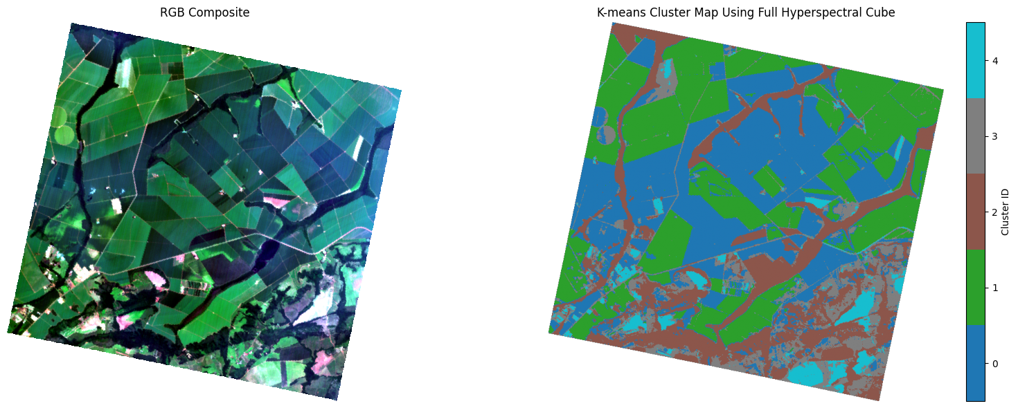
With K = 5, the clustering algorithm has identified five distinct spectral groups across the scene. The spatial distribution shows clear patterns:
Agricultural fields are separated into distinct clusters, likely reflecting differences in crop type, growth stage, or soil background
Dense vegetation surrounding water bodies form their own cluster with consistent grouping along what appear to be waterways
Bright surfaces (possibly roads or bare soil) are grouped separately
The vegetation-dominated landscape shows multiple clusters, suggesting spectral variation within vegetated areas
These initial results demonstrate that K-means can identify meaningful spectral groups using the full hyperspectral information. Now, let’s explore how the result changes when K-means uses only the RGB bands.
K-means Using RGB Bands Only
RGB clustering is a useful baseline because it shows what can be separated using only visible color information.
# Select RGB band indices from the list of cleaned wavelengths:
# - The nearest_band function finds the band index closest to the desired wavelength.
rgb_indices = [
    nearest_band(wavelengths_clean, 680),  # Red channel
    nearest_band(wavelengths_clean, 560),  # Green channel
    nearest_band(wavelengths_clean, 470),  # Blue channel
]

# Create the RGB feature matrix (X_rgb) by extracting the RGB band values for all valid pixels.
# This forms a (n_valid_pixels, 3) matrix for clustering with K-means.
X_rgb = X_valid[:, rgb_indices]

# Run K-means clustering using only the RGB bands and plot the resulting cluster map.
kmeans_rgb_map, labels_valid_rgb, kmeans_rgb = run_and_plot_kmeans(
    X_rgb,
    valid_mask,
    image_shape,
    N_CLUSTERS,
    RANDOM_STATE,
    cube_clean,
    wavelengths_clean,
    plot_title="K-means Cluster Map Using RGB Bands"
)
K-means completed with 5 clusters
Interpreting the RGB Results
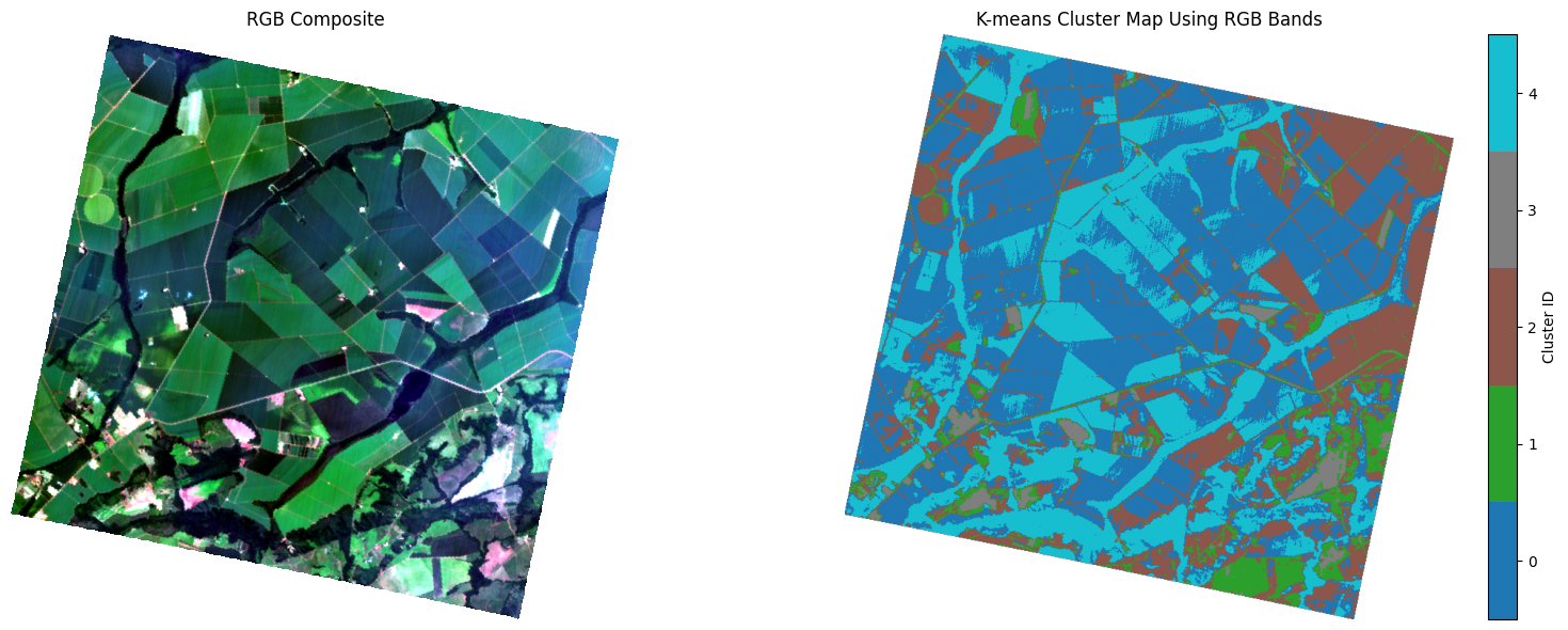
The RGB-based clustering shows considerably more noise and the clusters are not as spatially cohesive when compared to the full hyperspectral result. With only three bands, K-means has limited spectral information to distinguish between land-cover types. Materials with similar visible colors but different compositions (such as different crop types or vegetation conditions) cannot be separated effectively using RGB data alone.
Let’s compare the full hyperspectral clustering with the RGB-only result to see this difference more clearly.
# Compare full hyperspectral vs RGB clustering
plot_cluster_maps(
    maps=[kmeans_full_map, kmeans_rgb_map],
    titles=["K-means Using All Bands", "K-means Using RGB Bands"],
    N_CLUSTERS=N_CLUSTERS,
    separate_colorbars=True
)
(<Figure size 1400x600 with 4 Axes>,
 array([<Axes: title={'center': 'K-means Using All Bands'}>,
        <Axes: title={'center': 'K-means Using RGB Bands'}>], dtype=object))
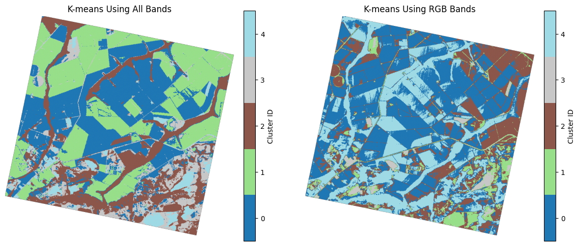
The side-by-side comparison reveals the limitation of RGB clustering. With only three bands, many agricultural fields fragment into multiple clusters or merge incorrectly with neighboring areas. This happens because RGB cannot distinguish materials with similar visible colors but different near-infrared or shortwave-infrared reflectance—such as crops at different growth stages or vegetation with varying water content.
The full hyperspectral result maintains more consistent cluster assignments because it uses spectral information across the visible, NIR, and SWIR regions.
Next, let’s examine whether PCA can achieve similar clustering quality while reducing dimensionality.
K-means Using PCA Components
PCA can reduce noise and dimensionality before clustering. This often speeds up K-means and can reduce the influence of weak or noisy bands.
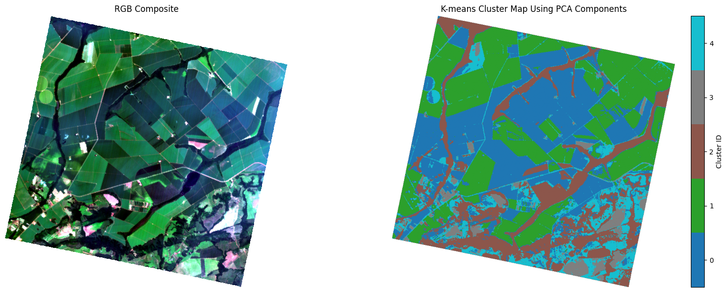
We’ll use the first 3 PCA components as the feature space for K-means.
# Number of PCA components to use for clustering (we use first 3 components)
PCA_COMPONENTS_FOR_CLUSTERING = 3

# Run PCA on the valid spectral pixels (no scaling here)
X_pca, pca_model, pca_scaler = run_pca(
    X_valid,
    n_components=PCA_COMPONENTS_FOR_CLUSTERING,
    scale=False,
    random_state=RANDOM_STATE,
)

# Print the shape of the new feature matrix (n_samples, n_components)
print(f"PCA feature matrix shape: {X_pca.shape}")

# Show the explained variance for each principal component
print("Explained variance ratio:")
for i, ratio in enumerate(pca_model.explained_variance_ratio_, start=1):
    print(f"PC{i}: {ratio:.4f}")

# Print total variance explained by all chosen components
print(f"Total explained variance: {pca_model.explained_variance_ratio_.sum():.4f}")
PCA feature matrix shape: (422557, 3)
Explained variance ratio:
PC1: 0.7486
PC2: 0.2347
PC3: 0.0071
Total explained variance: 0.9904
# Run K-means clustering on the PCA-transformed data and plot the resulting cluster map
kmeans_pca_map, labels_valid_pca, kmeans_pca = run_and_plot_kmeans(
    X_pca,
    valid_mask,
    image_shape,
    N_CLUSTERS,
    RANDOM_STATE,
    cube_clean,
    wavelengths_clean,
    plot_title="K-means Cluster Map Using PCA Components"
)
K-means completed with 5 clusters
Let’s compare the full hyperspectral clustering with the PCA-based result.
# Compare full hyperspectral vs PCA clustering
plot_cluster_maps(
    maps=[kmeans_full_map, kmeans_pca_map],
    titles=["K-means Using All Bands", "K-means Cluster Map Using PCA Components"],
    N_CLUSTERS=N_CLUSTERS,
    separate_colorbars=True
)
(<Figure size 1400x600 with 4 Axes>,
 array([<Axes: title={'center': 'K-means Using All Bands'}>,
        <Axes: title={'center': 'K-means Cluster Map Using PCA Components'}>],
       dtype=object))
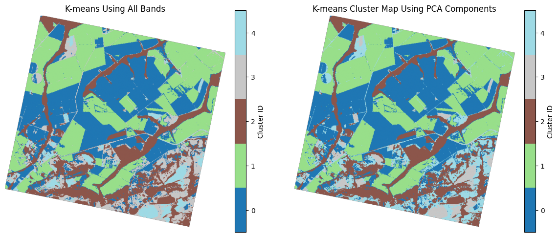
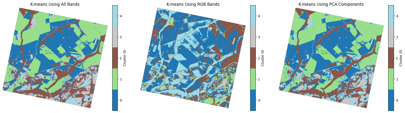
The K-means results of the full hyperspectral cube against those from PCA components are very similar. Only slight pixel-level differences appear between the two results (after you account for different cluster IDs and assigned colors). This suggests that the first three PCA components preserved most of the important spectral information needed for clustering, while reducing the dimensionality of the data.
Let’s put the three results side by side and write the final conclusion.
# Compare all three clustering approaches
plot_cluster_maps(
    maps=[kmeans_full_map, kmeans_rgb_map, kmeans_pca_map],
    titles=["K-means Using All Bands", "K-means Using RGB Bands", "K-means Using PCA Components"],
    N_CLUSTERS=N_CLUSTERS,
    separate_colorbars=True
)
(<Figure size 2100x600 with 6 Axes>,
 array([<Axes: title={'center': 'K-means Using All Bands'}>,
        <Axes: title={'center': 'K-means Using RGB Bands'}>,
        <Axes: title={'center': 'K-means Using PCA Components'}>],
       dtype=object))
Comparing the three K-means results shows how the input data affects the clustering quality. The result using all hyperspectral bands produces the most meaningful spatial pattern, where the clusters separate different land-cover conditions more clearly.
The RGB-based result is less consistent. Many fields are split into several clusters, and some areas are shifted into different groups. This happens because RGB bands contain only limited visible information, so materials with similar colors are difficult to separate.
The result using PCA components is closer to the full hyperspectral result. Although some pixel-level differences appear, the main spatial patterns and land-cover separations are still preserved. This shows that PCA keeps most of the important spectral information for clustering this scene while reducing the number of bands.
Overall, this comparison shows that hyperspectral data provide richer information than RGB for K-means clustering. PCA can also be an effective alternative because it reduces data dimensionality while maintaining most of the useful spectral variation.
To confirm this visual interpretation, we can also compare the cluster maps quantitatively using similarity metrics such as Adjusted Rand Index and Normalized Mutual Information, which will show how close the RGB-based and PCA-based results are to the full hyperspectral result.
First, though, we’ll pause to better understand some preprocessing decisions critical to clustering analysis.
Understanding the Role of Preprocessing and Normalization
Now that you’ve seen how different input features affect clustering results, let’s explore the preprocessing decisions in more depth. Understanding these choices will help you make better decisions when applying K-means to your own hyperspectral data.
General Preprocessing Framework
Before applying K-means to hyperspectral data, a systematic preprocessing workflow should include:
Define the objective - What should the clusters represent? Land-cover types, crop conditions, moisture differences?
Remove bad or noisy bands - Exclude bands affected by low signal-to-noise ratio, atmospheric absorption, or water vapor regions.
Mask invalid or irrelevant pixels - Exclude clouds, shadows, no-data pixels, and areas outside the study region.
Decide whether brightness should matter - Raw reflectance contains both brightness and spectral shape. Is one or both important for your application?
Choose an appropriate normalization method - This determines what kind of spectral differences K-means will emphasize.
Consider dimensionality reduction - PCA or other methods can reduce noise and improve computational efficiency.
Interpret and validate - Use spectral profiles, spatial patterns, field knowledge, and reference data to evaluate results.
The Normalization Decision
Quantitative comparison of cluster maps
Because K-means cluster IDs are arbitrary, we cannot compare the maps by simply checking whether the label numbers are the same. For example, Cluster 1 in one map may correspond to Cluster 3 in another map. Therefore, we use permutation-invariant metrics that measure similarity between cluster maps without depending on the exact cluster ID numbers.
Adjusted Rand Index (ARI): Measures how similarly pairs of pixels are grouped in two maps. A value of 1 means perfect agreement, while values close to 0 indicate agreement similar to random clustering.
Normalized Mutual Information (NMI): Measures how much information is shared between two clustering results. A value of 1 means the two maps contain almost the same clustering information.
In this comparison, the full-cube K-means result is used as the reference because it contains all the bands (i.e., all possible information). The RGB-based and PCA-based clustering maps are compared against it. These metrics help us quantify how similar the cluster maps are, but they do not prove that one clustering result is the true or scientifically correct classification. They only measure agreement between different clustering outputs.
def compare_cluster_maps(reference_map, target_map):
    """
    Compare two cluster maps using permutation-invariant similarity metrics.

    Because K-means assigns cluster IDs arbitrarily, we cannot directly compare
    cluster labels between two independent runs. Instead, this function uses
    metrics that measure clustering agreement regardless of how the clusters
    are numbered.

    Parameters
    ----------
    reference_map : ndarray, shape (rows, cols)
        First cluster map (typically the baseline for comparison).
    target_map : ndarray, shape (rows, cols)
        Second cluster map to compare against the reference.

    Returns
    -------
    metrics : dict
        Dictionary containing:
        - 'adjusted_rand_index': Measures similarity of pixel groupings.
          Values range from -1 to 1, where 1 = perfect agreement,
          0 = random clustering, negative = worse than random.
        - 'normalized_mutual_information': Measures shared information
          between clusterings. Values range from 0 to 1, where
          1 = identical clustering structure, 0 = no shared information.

    Notes
    -----
    - Both maps must have the same shape.
    - NaN and inf values are automatically excluded from the comparison.
    - Only pixels that are valid (finite) in BOTH maps are used.
    """
    # Flatten both maps to 1D arrays
    ref = reference_map.ravel()
    tgt = target_map.ravel()

    # Keep only pixels that are finite (not NaN, not inf) in both maps
    valid = np.isfinite(ref) & np.isfinite(tgt)
    ref_comp = ref[valid]
    tgt_comp = tgt[valid]

    return {
        "adjusted_rand_index": adjusted_rand_score(ref_comp, tgt_comp),
        "normalized_mutual_information": normalized_mutual_info_score(ref_comp, tgt_comp),
    }
# Run comparisons between the full hyperspectral K-means map and the RGB and PCA maps

# Initialize an empty list to store comparison results for each pair of cluster maps
comparison_rows = []

# Loop through the pairs of cluster maps to compare and compute similarity metrics
for name, cluster_map in [
    ("RGB vs all bands", kmeans_rgb_map),
    ("PCA vs all bands", kmeans_pca_map),
]:
    scores = compare_cluster_maps(kmeans_full_map, cluster_map)
    comparison_rows.append({"comparison": name, **scores})

# Create a DataFrame from the comparison results and display it
comparison_df = pd.DataFrame(comparison_rows)
comparison_dfThe quantitative results support our previous visual comparison. The RGB vs all bands comparison has a low ARI value of 0.232 and a low NMI value of 0.349, which means the RGB-based clustering has weak agreement with the full hyperspectral clustering. This confirms that using only RGB bands loses a large amount of spectral information, causing many pixels and fields to be grouped differently.
In contrast, the PCA vs all bands comparison shows extremely high agreement, with an ARI of 0.996 and an NMI of 0.991. This means the PCA-based clustering is almost identical to the clustering obtained from the full hyperspectral cube. Therefore, PCA successfully preserves the most important spectral information needed for K-means clustering while reducing the number of input bands.
Overall, these results show that RGB is not sufficient to reproduce the full hyperspectral clustering, while PCA provides a very close approximation to the full-band result.
After comparing the cluster maps visually and quantitatively, the next step is to look more deeply at why the PCA-based K-means result is so close to the full hyperspectral result. To do this, we examine the data in the PCA feature space using the first two principal components, PC1 and PC2.
These two components summarize the main spectral variation in the hyperspectral cube. By plotting the pixels in PC1–PC2 space, we can see how the K-means clusters are separated and where the cluster centers are located. We can also compare this with the PC1 and PC2 image maps to understand what kind of spatial and spectral information each component captures.
This analysis helps explain how PCA reduces the hyperspectral data into fewer dimensions while still preserving the most important information needed for clustering.
PCA Feature-Space Diagnostics for K-means Clustering
The diagnostic visualization below shows how pixels are distributed in PC1–PC2 space, along with the K-means cluster centers, spatial maps of each component, and the final cluster map.
If clusters are well separated in PCA space and their spatial patterns align with field boundaries, then the first two principal components captured the spectral variation that drives clustering in the full hyperspectral data.
def plot_pca_2d_clustering_diagnostics(
    X_pca,
    labels_valid_pca,
    kmeans_pca,
    kmeans_pca_map,
    pc1_map,
    pc2_map,
    n_clusters
):
    """
    Visualize K-means clustering results in PCA feature space with diagnostic plots.

    Creates a 6-panel figure showing:
    - Scatter plot of pixels in PC1-PC2 space with cluster assignments
    - False-color composite of PC1 and PC2
    - Spatial cluster map
    - Individual PC1 and PC2 spatial maps

    Parameters
    ----------
    X_pca : ndarray, shape (n_pixels, 2)
        PCA-transformed data (first 2 components).
    labels_valid_pca : ndarray
        Cluster labels for each pixel.
    kmeans_pca : KMeans
        Fitted KMeans object.
    kmeans_pca_map : ndarray, shape (rows, cols)
        2D cluster map.
    pc1_map : ndarray, shape (rows, cols)
        Spatial map of PC1.
    pc2_map : ndarray, shape (rows, cols)
        Spatial map of PC2.
    n_clusters : int
        Number of clusters.

    Returns
    -------
    fig : Figure
        Matplotlib figure object.
    axes : ndarray
        Array of axes objects.
    """

    def normalize(arr):
        low, high = np.nanpercentile(arr, [2, 98])
        return np.clip((arr - low) / (high - low), 0, 1)

    cmap = plt.get_cmap("tab10", n_clusters)

    pca_rgb = np.dstack([
        normalize(pc1_map),
        normalize(pc2_map),
        np.zeros_like(pc1_map)
    ])

    fig, axes = plt.subplots(2, 3, figsize=(18, 10))

    ax = axes[0, 0]
    ax.scatter(
        X_pca[:, 0],
        X_pca[:, 1],
        c=labels_valid_pca,
        cmap=cmap,
        s=4,
        alpha=0.5
    )
    ax.scatter(
        kmeans_pca.cluster_centers_[:, 0],
        kmeans_pca.cluster_centers_[:, 1],
        c="black",
        s=150,
        marker="X",
        label="Centers"
    )
    ax.set(
        title="K-means clusters in PCA space",
        xlabel="PC1",
        ylabel="PC2"
    )
    ax.legend()

    axes[0, 1].imshow(pca_rgb)
    axes[0, 1].set_title("False-color composite: PC1 (red), PC2 (green)")

    im = axes[0, 2].imshow(
        np.ma.masked_invalid(kmeans_pca_map),
        cmap=cmap,
        vmin=-0.5,
        vmax=n_clusters - 0.5
    )
    axes[0, 2].set_title("Spatial K-means map from PCA features")
    fig.colorbar(im, ax=axes[0, 2], ticks=range(n_clusters), label="Cluster ID")

    axes[1, 0].imshow(pc1_map, cmap="gray")
    axes[1, 0].set_title("PC1 spatial map")

    axes[1, 1].imshow(pc2_map, cmap="gray")
    axes[1, 1].set_title("PC2 spatial map")

    for ax in axes.ravel()[1:]:
        ax.axis("off")

    plt.tight_layout()
    plt.show()

    return fig, axes
# Select the first two PCA components for clustering
X_pca_2 = X_pca[:, :2]
# Run K-means clustering using only PC1 and PC2
kmeans_pca2_map, labels_valid_pca2, kmeans_pca2 = run_and_plot_kmeans(
X_pca_2,
valid_mask,
image_shape,
N_CLUSTERS,
RANDOM_STATE,
cube_clean,
wavelengths_clean,
plot_title="K-means Cluster Map Using First 2 PCA Components"
)
# Reconstruct spatial maps for PC1 and PC2 (needed for diagnostic visualization)
# Create an array to hold all pixels (valid + invalid) for both components
pca_2comp_full = np.full(
(valid_mask.ravel().shape[0], 2),
np.nan,
dtype=np.float32
)
# Fill in the valid pixel locations with their PC1 and PC2 values
pca_2comp_full[valid_mask.ravel()] = X_pca_2
# Reshape from flat array back to 2D image with 2 channels (PC1, PC2)
pca_2comp_maps = pca_2comp_full.reshape(
image_shape[0],
image_shape[1],
2
)
# Extract individual spatial maps for PC1 and PC2
pc1_2comp_map = pca_2comp_maps[:, :, 0]
pc2_2comp_map = pca_2comp_maps[:, :, 1]
print(f"PCA 2-component maps shape: {pca_2comp_maps.shape}")K-means completed with 5 clusters
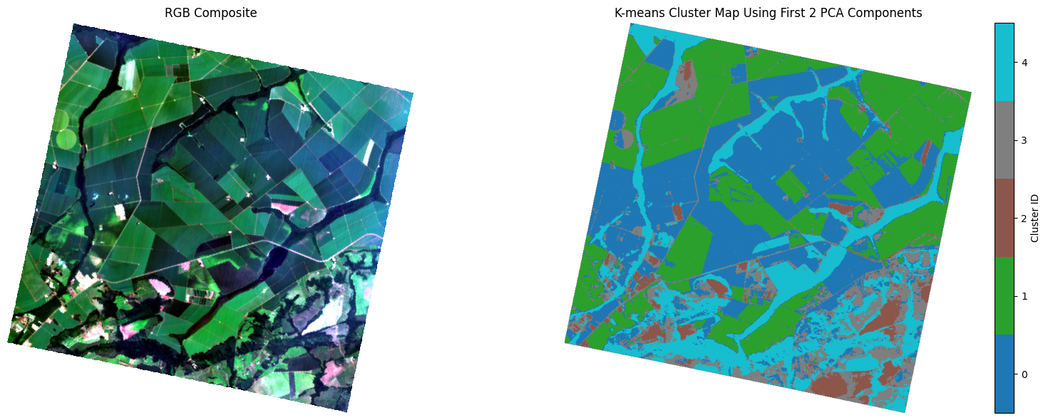
PCA 2-component maps shape: (752, 784, 2)
fig, axes = plot_pca_2d_clustering_diagnostics(
    X_pca=X_pca_2,
    labels_valid_pca=labels_valid_pca2,
    kmeans_pca=kmeans_pca2,
    kmeans_pca_map=kmeans_pca2_map,
    pc1_map=pc1_2comp_map,
    pc2_map=pc2_2comp_map,
    n_clusters=N_CLUSTERS
)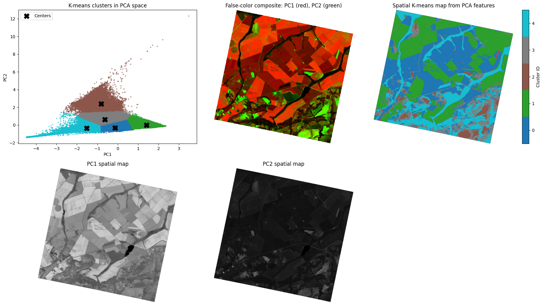
The cluster centers are well distributed across the PCA space, showing that K-means is finding distinct spectral groups rather than assigning pixels randomly.
The point cloud has a fan-like/triangular shape because PC1 and PC2 are linear combinations of the original hyperspectral bands. PCA compresses the majority of the data variance into only two linear axes, so complex spectral relationships are projected into a simplified 2D feature space. This can make some clusters overlap near the center, especially for mixed pixels or transitional areas where spectral differences are weak.
This also highlights a limitation of PCA: it is a linear dimensionality reduction method, so it may not fully capture non-linear spectral patterns in hyperspectral data (of which there can be many!). For more complex structures, non-linear methods such as t-SNE, UMAP, or autoencoders may reveal separations that PCA cannot show clearly. You can see an example of UMAP results at the end of the dimensionality reduction lesson.
Be careful with Elbow and Silhouette scores
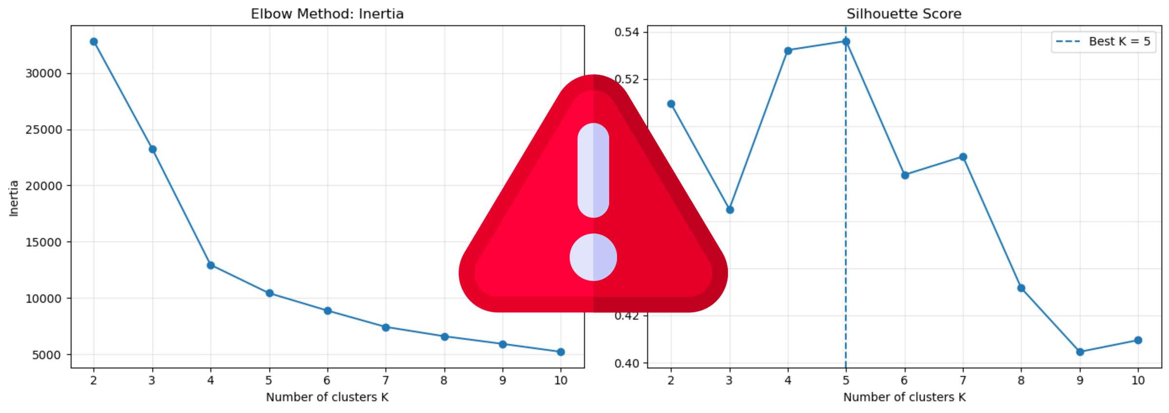
Figure 3:Elbow and silhouette diagnostics for selecting the number of clusters in hyperspectral K-means. These scores must be interpreted carefully alongside spectral and spatial knowledge.
As shown in Figure 3, in hyperspectral clustering, you may use diagnostic plots and scores to better understand the “optimal” number of clusters. However, inertia and silhouette scores can be misleading. The elbow curve may not show a clear break, and the silhouette score may suggest a value of K that is not meaningful in relation to the actual land-cover classes present in an image.
This happens because hyperspectral data are high-dimensional and can be highly correlated. Pixels often contain mixed materials and have varying illumination effects and within-class spectral variability.
Therefore, the “best” number of clusters should not be selected only from these numerical scores. Instead, K should be chosen using spectral interpretation, including the mean spectral signature of each cluster, spatial consistency, field knowledge, and comparison with ground reference data.
Choosing K using spectral interpretation
Instead of relying only on inertia or silhouette scores, we can examine how the mean spectral signatures change as the number of clusters increases.
In this step, K-means is run for different values of K from 2 to 10. For each K, we plot:
the mean spectrum of each cluster,
the spectral variability within each cluster using ±1 standard deviation,
the number of pixels assigned to each cluster.
This helps us understand whether increasing K creates meaningful new spectral groups or only splits existing clusters into small or noisy groups.
A good value of K should produce clusters with distinct spectral signatures, reasonable pixel counts, and meaningful spatial patterns. The goal is not just to maximize a score, but to choose a K that makes sense from a hyperspectral and land-cover interpretation point of view.
# Multi-K spectral signature plot + cluster pixel-count bars
# This creates a grid of plots showing how spectral signatures and cluster sizes change as K varies from 2 to 10

k_values_to_explore = [2, 3, 4, 5, 6, 7, 8, 9, 10]

n_rows = len(k_values_to_explore)

fig, axes = plt.subplots(
    n_rows,
    2,
    figsize=(17, 4.8 * n_rows),
    gridspec_kw={"width_ratios": [3, 1.2]}
)

# Use tab10 colormap, allowing up to 10 unique colors
colors_palette = plt.get_cmap("tab10").colors

for ax_idx, k in enumerate(k_values_to_explore):

    ax_spec = axes[ax_idx, 0]
    ax_bar = axes[ax_idx, 1]

    # Fit K-means for the current value of K
    km = KMeans(n_clusters=k, random_state=RANDOM_STATE, n_init="auto")
    km.fit(X_valid)
    labels_k = km.predict(X_valid)

    cluster_counts = []

    # For each cluster, compute and plot the mean spectrum with ±1 std dev shading
    for cid in range(k):
        mask_c = labels_k == cid
        cluster_spectra = X_valid[mask_c]

        # Calculate mean and standard deviation of spectral signatures for this cluster
        mean_spec = np.mean(cluster_spectra, axis=0)
        std_spec = np.std(cluster_spectra, axis=0)

        cluster_count = mask_c.sum()
        cluster_counts.append(cluster_count)

        color = colors_palette[cid % len(colors_palette)]

        ax_spec.plot(
            wavelengths_clean,
            mean_spec,
            color=color,
            linewidth=1.8,
            label=f"C{cid} (n={cluster_count:,})"
        )

        ax_spec.fill_between(
            wavelengths_clean,
            mean_spec - std_spec,
            mean_spec + std_spec,
            color=color,
            alpha=0.15
        )

    # Spectral plot formatting
    ax_spec.set_title(
        f"K = {k}: Mean Spectrum ± 1 Std Dev",
        fontsize=13,
        fontweight="bold"
    )
    ax_spec.set_xlabel("Wavelength (nm)", fontsize=10)
    ax_spec.set_ylabel("Reflectance", fontsize=10)
    ax_spec.grid(alpha=0.2)
    ax_spec.legend(fontsize=8, loc="upper right")

    # Bar plot: number of pixels per cluster
    cluster_ids = np.arange(k)
    bar_colors = [colors_palette[cid % len(colors_palette)] for cid in cluster_ids]

    bars = ax_bar.bar(
        cluster_ids,
        cluster_counts,
        color=bar_colors,
        edgecolor="black",
        alpha=0.85
    )

    ax_bar.set_title("Pixels per Cluster", fontsize=12, fontweight="bold")
    ax_bar.set_xlabel("Cluster ID", fontsize=10)
    ax_bar.set_ylabel("Number of Pixels", fontsize=10)
    ax_bar.set_xticks(cluster_ids)
    ax_bar.set_xticklabels([f"C{cid}" for cid in cluster_ids], rotation=45)
    ax_bar.grid(axis="y", alpha=0.2)

    # Give extra vertical space so labels are not cut off
    max_count = max(cluster_counts)
    ax_bar.set_ylim(0, max_count * 1.25)

    # Add pixel count labels above each bar (rotated 90° to save space)
    for bar, count in zip(bars, cluster_counts):
        ax_bar.text(
            bar.get_x() + bar.get_width() / 2,
            bar.get_height() + max_count * 0.02,
            f"{count:,}",
            ha="center",
            va="bottom",
            fontsize=9,
            rotation=90,
            bbox=dict(
                facecolor="white",
                edgecolor="none",
                alpha=0.75,
                pad=1.5
            )
        )

plt.suptitle(
    "How Clusters 'Split' as K Increases\nMean Spectrum ± 1 Std Dev and Pixel Count per Cluster",
    fontsize=15,
    fontweight="bold",
    y=0.995)

plt.tight_layout()
plt.show()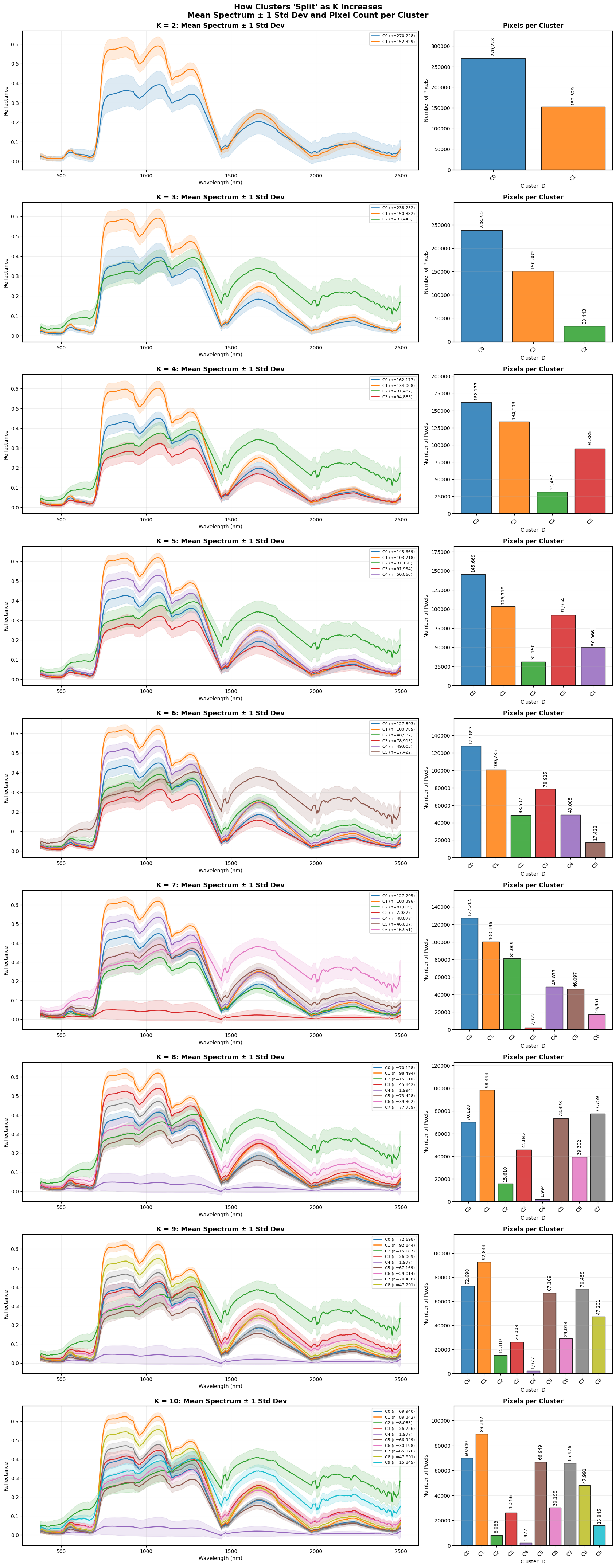
The multi-K spectral signature plots show that increasing the number of clusters does not only split the data numerically; it also reveals new spectral groups with different physical meaning. As K increases, some broad clusters begin to separate into more specific surface conditions, such as different vegetation states, soil/background variation, and wet or low-reflectance materials.
An important observation is that around K = 7, a distinct spectral signature related to water starts to appear. This suggests that smaller K values were merging water or wet areas with other low-reflectance surfaces, while higher K values allow K-means to isolate this material more clearly.
For this reason, we continued testing up to K = 10 to see whether additional meaningful spectral groups appear. The next step is to visualize the thematic cluster map for K = 10 and examine whether these spectral differences also form meaningful spatial patterns.
# Set the number of clusters to use for K-means
N_CLUSTERS = 10

kmeans_full_map, labels_valid_full, kmeans_full = run_and_plot_kmeans(
    X_valid,
    valid_mask,
    image_shape,
    N_CLUSTERS,
    RANDOM_STATE,
    cube_clean,
    wavelengths_clean,
    plot_title="K-means Cluster Map Using Full Hyperspectral Cube"
)
K-means completed with 10 clusters
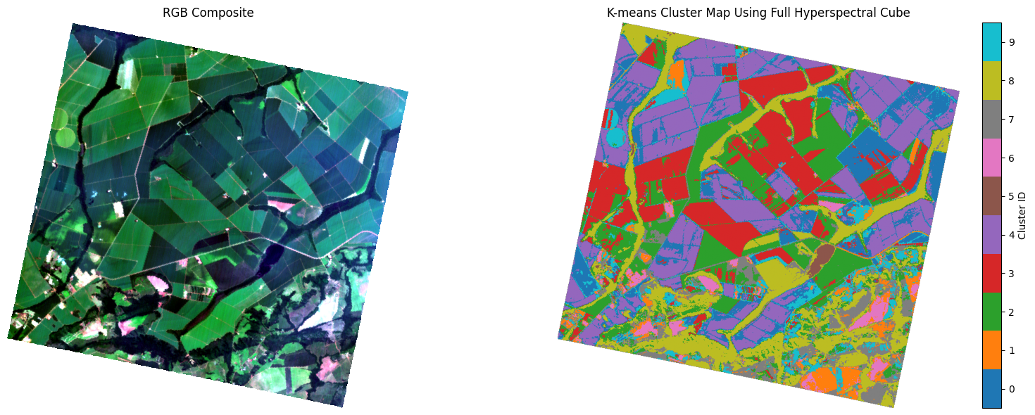
With K = 10 and the full hyperspectral cube, we can distinguish more variability in the scene. More detailed surface differences appear, including vegetation variation, soil/background differences, roads, and wet areas. Importantly, the deeper water is now separated more clearly and appears as the gray cluster, Cluster 7, on the map. This shows that increasing K can reveal meaningful spectral classes that were hidden or merged at lower K values.
Assignment
In the previous lesson, we learned how to reconstruct the PCA components to create a cleaner hyperspectral cube with reduced noise. Your assignment is to replicate what you learned in this lesson using the denoised hyperspectral cube and compare the results.
Beyond K-means: What’s Next?
K-means is a useful starting point, but it is only one way to cluster hyperspectral data. It is a hard clustering method, meaning each pixel is assigned to only one cluster.
In real hyperspectral images, this is not always realistic. A single pixel may contain a mixture of vegetation, soil, water, or shadow. This leads to other approaches:
Soft clustering, such as Gaussian Mixture Models, where a pixel can belong to multiple clusters with different probabilities.
Spectral unmixing, where each pixel is treated as a mixture of several pure materials, called endmembers.
Density-based clustering, such as DBSCAN, which can find irregular cluster shapes and identify noise or outliers.
These methods open the door to a deeper question: Are we trying to assign each pixel to one class, or understand what materials are mixed inside each pixel?
Recommended Resource
A great resource we recommend for learning more about unsupervised learning is the scikit-learn documentation. It provides clear explanations, examples, and practical implementations of clustering, dimensionality reduction, mixture models, and other unsupervised learning methods.
You can start here:
🧰 Your Complete Hyperspectral Toolkit
That’s a wrap on the build-your-own-toolkit thread. Over Modules 2–4 you grew a single, reusable library — from reading and cleaning a Tanager-1 cube, through band selection, spectral indices, dimensionality reduction and denoising, to unsupervised clustering.
The cell below collects the entire reference toolkit in one place. Keep it as your starting point for any new hyperspectral analysis — it’s yours now.
# ==================
# 🧰 YOUR COMPLETE TOOLKIT  (Modules 2–4 — the whole reference library)
# ==================

# Essential imports
import h5py as h5
import numpy as np
import matplotlib.pyplot as plt
import pandas as pd
from sklearn.cluster import KMeans
from sklearn.decomposition import PCA
from sklearn.preprocessing import StandardScaler
from sklearn.metrics import adjusted_rand_score, normalized_mutual_info_score


# Reproducibility for PCA / clustering
RANDOM_STATE = 31


# ---- setup -------------------------------------------------------------

def download_tanager_data(url, file_path):
    import os
    import urllib.request

    def _progress(count, block_size, total_size):
        mb_done = count * block_size / 1_000_000
        mb_total = total_size / 1_000_000
        print(f"\rDownloading... {mb_done:.1f} / {mb_total:.1f} MB", end="", flush=True)

    if not os.path.exists(file_path):
        urllib.request.urlretrieve(url, file_path, reporthook=_progress)
        print(f"\nDownload complete: {file_path}")
    else:
        print(f"File already exists, skipping download: {file_path}")
    return file_path


# ---- io ----------------------------------------------------------------

def print_structure(name, obj):
    level = name.count('/')
    indent = '    ' * level
    if isinstance(obj, h5.Group):
        print(f"{indent}📂 {name}/")
    elif isinstance(obj, h5.Dataset):
        print(f"{indent}📄 {name} | {obj.shape} | {obj.dtype}")
    if len(obj.attrs) > 0:
        for key, val in obj.attrs.items():
            val_str = str(val)
            if len(val_str) > 50:
                val_str = val_str[:50] + "..."
            print(f"{indent}    ↳ 🏷️ {key}: {val_str}")

def load_hdf5(
    file_path,
    data_path='HDFEOS/GRIDS/HYP/Data Fields/surface_reflectance',
    nodata_path='HDFEOS/GRIDS/HYP/Data Fields/nodata_pixels',
    clean=True,
    band=None
    ):

    with h5py.File(file_path, 'r') as f:
        dset = f[data_path]
        # select all or a single band
        if band is None:
            data = dset[:].astype(np.float32)
        else:
            data = dset[band].astype(np.float32)
        attrs = dict(dset.attrs)

        wavelengths = np.asarray(attrs['wavelengths'], dtype=np.float32)
        good = np.asarray(attrs['good_wavelengths'], dtype=bool)
        no_data = f[nodata_path][:].astype(bool)

    if clean:
        if band is None:
            data = data[good]
            wavelengths = wavelengths[good]
            data[:, no_data] = np.nan
            good = good[good]
        else:
            # For a single band, check if it is good, else return all nan
            wavelengths = np.array([wavelengths[band]], dtype=np.float32)
            if not good[band]:
                data = np.full_like(data, np.nan)
            else:
                data[no_data] = np.nan
            good = np.array([good[band]], dtype=bool)

    attrs['wavelengths'] = wavelengths
    attrs['good_wavelengths'] = good

    return data, attrs, no_data


# ---- bands -------------------------------------------------------------

def nearest_band(wavelengths, target_nm):
    """Return the index of the band whose wavelength is closest to ``target_nm``."""
    return int(np.argmin(np.abs(np.asarray(wavelengths) - target_nm)))

def get_band(cube, wavelengths, target_nm, verbose=True):
    """Return the 2-D band nearest ``target_nm`` (uses ``nearest_band``).

    Parameters
    ----------
    cube : ndarray, shape (bands, rows, cols)
        Hyperspectral cube.
    wavelengths : ndarray
        Per-band center wavelengths (nm).
    target_nm : float
        Requested wavelength (nm).
    verbose : bool, optional
        If True, print the actual wavelength used and its shift from the request.

    Returns
    -------
    ndarray, shape (rows, cols)
        The 2-D band nearest ``target_nm``.
    """
    idx = nearest_band(wavelengths, target_nm)
    actual_nm = float(wavelengths[idx])
    if verbose:
        print(
            f"Requested {target_nm} nm -> using {actual_nm:.2f} nm "
            f"(shift: {actual_nm - target_nm:+.2f} nm)"
        )
    return cube[idx, :, :]

def select_wavelengths(wavelengths, min_nm=None, max_nm=None, exclude_ranges=None):
    """Return a Boolean mask for wavelengths to keep.

    Parameters
    ----------
    wavelengths : ndarray
        Array of wavelength values in nanometers.
    min_nm : float, optional
        Minimum wavelength to keep (inclusive).
    max_nm : float, optional
        Maximum wavelength to keep (inclusive).
    exclude_ranges : list of tuples, optional
        List of (low, high) wavelength ranges to exclude.

    Returns
    -------
    keep : ndarray, dtype=bool
        Boolean mask where True indicates wavelengths to keep.
    """
    keep = np.ones_like(wavelengths, dtype=bool)
    if min_nm is not None:
        keep &= wavelengths >= min_nm
    if max_nm is not None:
        keep &= wavelengths <= max_nm
    if exclude_ranges is not None:
        for low, high in exclude_ranges:
            keep &= ~((wavelengths >= low) & (wavelengths <= high))
    return keep


# ---- transform ---------------------------------------------------------


def flatten_cube(cube, no_data=None):
    bands, rows, cols = cube.shape
    X = cube.reshape(bands, rows * cols).T
    valid_mask = np.isfinite(X).all(axis=1)
    if no_data is not None:
        valid_mask &= ~no_data.ravel()
    X_valid = X[valid_mask]
    return X, X_valid, valid_mask

def run_pca(X, n_components=10, scale=False, random_state=RANDOM_STATE):
    scaler = None
    X_input = X
    if scale:
        scaler = StandardScaler()
        X_input = scaler.fit_transform(X)
    pca_model = PCA(n_components=n_components, random_state=random_state)
    X_pca = pca_model.fit_transform(X_input)
    return X_pca, pca_model, scaler


# ---- visualization ----------------------------------------------------

def make_rgb(cube, wavelengths, r_nm=680, g_nm=550, b_nm=470,
             percentile_low=2, percentile_high=98, reference_cube=None):
    """Create a display RGB using per-channel percentile stretching.

    If `reference_cube` is provided, display limits are computed from both cubes
    so before/after RGB images use the same stretch.
    """
    r = nearest_band(wavelengths, r_nm)
    g = nearest_band(wavelengths, g_nm)
    b = nearest_band(wavelengths, b_nm)
    band_indices = (r, g, b)

    rgb = np.dstack([cube[idx] for idx in band_indices]).astype(np.float32)
    if reference_cube is None:
        stretch_rgb = rgb
    else:
        reference_rgb = np.dstack([reference_cube[idx] for idx in band_indices]).astype(np.float32)
        stretch_rgb = np.concatenate([rgb, reference_rgb], axis=0)

    rgb_display = np.zeros_like(rgb, dtype=np.float32)
    for channel in range(3):
        p_low, p_high = np.nanpercentile(
            stretch_rgb[:, :, channel],
            (percentile_low, percentile_high)
        )
        if not np.isfinite(p_low) or not np.isfinite(p_high) or p_high <= p_low:
            continue
        rgb_display[:, :, channel] = (rgb[:, :, channel] - p_low) / (p_high - p_low)

    return np.clip(rgb_display, 0, 1)

def contrast_stretching(image, lower=2, upper=98):
    """Return display limits for contrast stretching based on percentiles."""
    return np.nanpercentile(image, lower), np.nanpercentile(image, upper)

def plot_index_with_hist(index_arr,
                        index_name="Index",
                        hist_label="Value",
                        cmap='RdYlGn',
                        figsize=(10, 6),
                        vmin=None,
                        vmax=None):
    arr = index_arr
    if vmin is None or vmax is None:
        vmin, vmax = contrast_stretching(arr)

    fig, axes = plt.subplots(1, 2, figsize=figsize, gridspec_kw={'width_ratios':[2,1]})

    im = axes[0].imshow(arr, cmap=cmap, vmin=vmin, vmax=vmax)
    axes[0].set_title(f"{index_name}", fontsize=14, fontweight='bold')
    axes[0].axis('off')
    plt.colorbar(im, ax=axes[0], fraction=0.046, pad=0.04, label=index_name)

    axes[1].hist(arr[~np.isnan(arr)].ravel(),
                 bins=500,
                 alpha=0.8,
                 range=(vmin, vmax), edgecolor='k')
    axes[1].set_title(f"{index_name} Histogram", fontsize=12)
    axes[1].set_xlabel(hist_label)
    axes[1].set_ylabel("Frequency")
    axes[1].grid(alpha=0.3)

    plt.tight_layout()
    plt.show()


# ---- spectral ----------------------------------------------------------

def spectral_sam(spec1, spec2):
    """Spectral Angle Mapper (radians) between two spectra. Lower = more similar."""
    mask = np.isfinite(spec1) & np.isfinite(spec2)
    if np.sum(mask) < 2:
        return np.nan
    a = spec1[mask]
    b = spec2[mask]
    denom = np.linalg.norm(a) * np.linalg.norm(b)
    if denom == 0:
        return np.nan
    cosang = np.clip(np.dot(a, b) / denom, -1, 1)
    return np.arccos(cosang)

def spectral_corr(spec1, spec2):
    """Pearson correlation between two spectra (-1..1; higher = more similar)."""
    mask = np.isfinite(spec1) & np.isfinite(spec2)
    if np.sum(mask) < 2:
        return np.nan
    a = spec1[mask]
    b = spec2[mask]
    if np.nanstd(a) == 0 or np.nanstd(b) == 0:
        return np.nan
    return np.corrcoef(a, b)[0, 1]

def spectral_mad(spec1, spec2):
    """Mean Absolute Difference between two spectra (reflectance units)."""
    diff = np.abs(spec1 - spec2)
    return np.nanmean(diff)

def sam_map(cube1, cube2, valid_mask=None):
    """Pixelwise Spectral Angle Mapper (radians) between two cubes -> 2-D map."""
    dot = np.nansum(cube1 * cube2, axis=0)
    norm1 = np.sqrt(np.nansum(cube1**2, axis=0))
    norm2 = np.sqrt(np.nansum(cube2**2, axis=0))
    denom = norm1 * norm2
    cosang = np.full_like(dot, np.nan, dtype=float)
    good = denom > 0
    cosang[good] = dot[good] / denom[good]
    cosang = np.clip(cosang, -1, 1)
    sam = np.arccos(cosang)
    if valid_mask is not None:
        sam[~valid_mask] = np.nan
    return sam


# ---- clustering --------------------------------------------------------

def run_kmeans_clustering(X_valid, n_clusters=5, random_state=None, n_init=10):
    """Fit KMeans on the valid pixels; returns (labels_valid, kmeans)."""
    kmeans = KMeans(n_clusters=n_clusters, random_state=random_state, n_init=n_init)
    labels_valid = kmeans.fit_predict(X_valid)
    print(f"K-means completed with {n_clusters} clusters")
    return labels_valid, kmeans

def labels_to_map(labels_valid, valid_mask, image_shape, invalid_label=np.nan):
    """Scatter 1-D cluster labels back into a 2-D image map (invalid pixels = NaN)."""
    valid_mask_flat = valid_mask.ravel()
    labels_full = np.full(valid_mask_flat.shape[0], invalid_label, dtype=float)
    labels_full[valid_mask_flat] = labels_valid
    return labels_full.reshape(image_shape)

def plot_kmeans_cluster_map(cluster_map, n_clusters, cube, wavelengths, title="K-means Cluster Map"):
    """Plot the RGB composite (via make_rgb) next to a K-means cluster map."""
    rgb_img = make_rgb(cube, wavelengths)
    fig, axes = plt.subplots(1, 2, figsize=(16, 6))
    axes[0].imshow(rgb_img)
    axes[0].set_title("RGB Composite", fontsize=12)
    axes[0].axis("off")
    cmap = plt.get_cmap("tab10", n_clusters).copy()
    img = axes[1].imshow(np.ma.masked_invalid(cluster_map), cmap=cmap,
                         vmin=-0.5, vmax=n_clusters - 0.5)
    axes[1].set_title(title, fontsize=12)
    axes[1].axis("off")
    cbar = fig.colorbar(img, ax=axes[1], ticks=range(n_clusters), fraction=0.046, pad=0.04)
    cbar.set_label("Cluster ID")
    plt.tight_layout()
    plt.show()

def run_and_plot_kmeans(X, valid_mask, image_shape, n_clusters, random_state,
                        cube, wavelengths, plot_title="K-means Cluster Map"):
    """Run K-means, map labels back to image space, and plot; returns (map, labels, kmeans)."""
    labels_valid, kmeans = run_kmeans_clustering(
        X_valid=X, n_clusters=n_clusters, random_state=random_state, n_init=10)
    kmeans_map = labels_to_map(labels_valid=labels_valid, valid_mask=valid_mask,
                               image_shape=image_shape)
    plot_kmeans_cluster_map(kmeans_map, n_clusters, cube, wavelengths, title=plot_title)
    return kmeans_map, labels_valid, kmeans

def plot_cluster_maps(maps, titles=None, N_CLUSTERS=5, cmap_name="tab20",
                      figsize_scale=(7, 6), colorbar_label="Cluster ID",
                      show=True, separate_colorbars=False):
    """Plot any number of cluster maps side by side (shared or separate colorbars)."""
    n_maps = len(maps)
    if titles is None:
        titles = [f"Map {i+1}" for i in range(n_maps)]
    elif len(titles) < n_maps:
        titles = titles + [f"Map {i+1}" for i in range(len(titles), n_maps)]
    fig, axes = plt.subplots(1, n_maps, figsize=(figsize_scale[0]*n_maps, figsize_scale[1]))
    if n_maps == 1:
        axes = [axes]
    cmap = plt.get_cmap(cmap_name, N_CLUSTERS).copy()
    imshow_kwargs = {"cmap": cmap, "vmin": -0.5, "vmax": N_CLUSTERS - 0.5}
    ims = []
    for i, (m, ax) in enumerate(zip(maps, axes)):
        im = ax.imshow(np.ma.masked_invalid(m), **imshow_kwargs)
        ax.set_title(titles[i])
        ax.axis("off")
        ims.append(im)
        if separate_colorbars:
            cbar = fig.colorbar(im, ax=ax, ticks=range(N_CLUSTERS), fraction=0.046, pad=0.04)
            cbar.set_label(colorbar_label)
    if not separate_colorbars:
        cbar = fig.colorbar(ims[-1], ax=axes, ticks=range(N_CLUSTERS), fraction=0.046, pad=0.04)
        cbar.set_label(colorbar_label)
    if show:
        plt.show()
    return fig, axes