
Welcome to Lesson 1 of Module 4 — Part 2. This part is the hands-on companion to Part 1. If you have not yet read Part 1, it covers the conceptual and theoretical foundations, why spectral indices are needed, how NDVI and EVI were developed, and how hyperspectral data enables more precise analysis. Here, you will apply those concepts to two real Tanager-1 scenes: an agricultural landscape in Campo Verde, Brazil, and a water body scene in Gwan-ri, South Korea.
Practical Application: Calculating Narrow-band Indices
For the vegetation and water-body applications, we use two Planet Tanager-1 scenes available through the open STAC catalog. The first scene covers an area of intensive agricultural production, making it well suited for exploring vegetation structure, vigor, and crop-related spectral variation. The second scene contains extensive water bodies with interconnected land and water surfaces, which makes it useful for examining water-related spectral behavior and land–water interactions. The two scenes used in this practical are shown below.
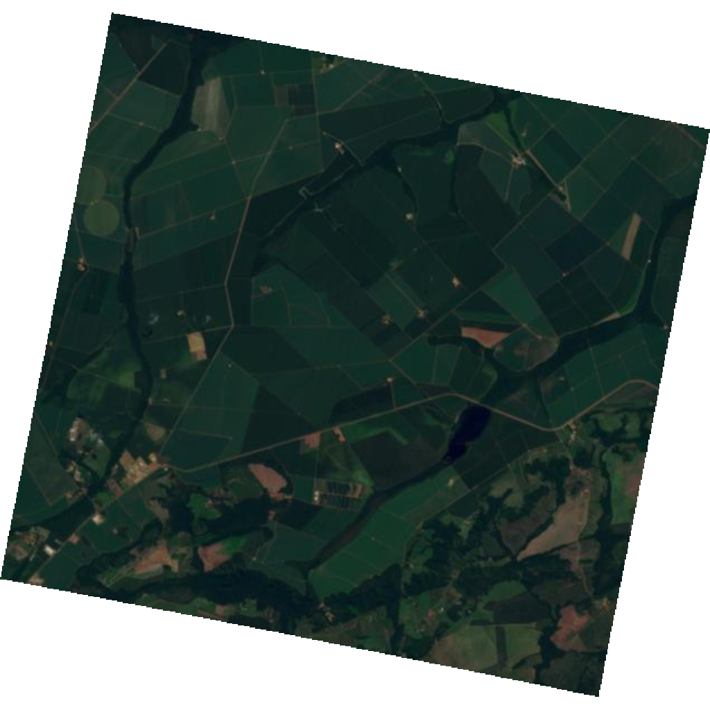
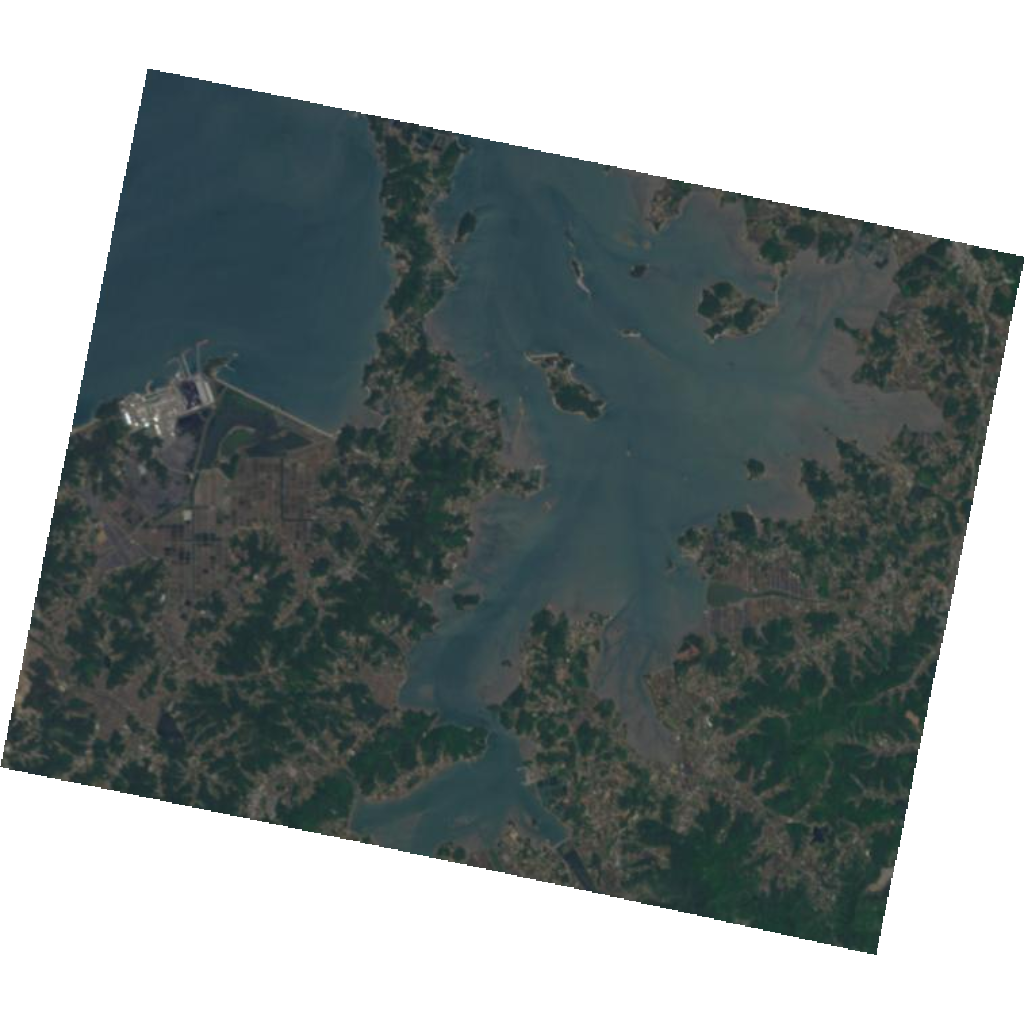
| Scene | Application | Time of Data | Location Description |
|---|---|---|---|
| 20250501_143138_87_4001 | Vegetation | 5/1/2025, 2:31:38 PM UTC | Campo Verde, Região Geográfica Imediata de Cuiabá, Região Metropolitana do Vale do Rio Cuiabá, Região Geográfica Intermediária de Cuiabá, Mato Grosso, Central-West Region, 78840-000, Brazil |
| 20250504_025815_32_4001 | Water Bodies | 5/4/2025, 2:58:15 AM UTC | Gwan-ri, Taean-gun, South Chungcheong, 32103, South Korea |
Setup and Helper Functions
To begin, we will prepare the environment and ensure that the specific scenes from the Tanager-1 Open STAC collection are available. The following cells will download the sample datasets and import all necessary libraries.
🧰 Your Toolkit so far
This is the reference solution for everything you’ve built through Module 3 · Lesson 1, compare it with the versions you implemented as last lesson’s challenge (the cleaning load_hdf5).
# ==================
# 🧰 YOUR TOOLKIT
# ==================

# Essential imports
import h5py
import numpy as np
import matplotlib.pyplot as plt


# ---- setup -------------------------------------------------------------

def download_tanager_data(url, file_path):
    import os
    import urllib.request

    def _progress(count, block_size, total_size):
        mb_done = count * block_size / 1_000_000
        mb_total = total_size / 1_000_000
        print(f"\rDownloading... {mb_done:.1f} / {mb_total:.1f} MB", end="", flush=True)

    if not os.path.exists(file_path):
        urllib.request.urlretrieve(url, file_path, reporthook=_progress)
        print(f"\nDownload complete: {file_path}")
    else:
        print(f"File already exists, skipping download: {file_path}")
    return file_path


# ---- io ----------------------------------------------------------------

def load_hdf5(
    file_path,
    data_path='HDFEOS/GRIDS/HYP/Data Fields/surface_reflectance',
    nodata_path='HDFEOS/GRIDS/HYP/Data Fields/nodata_pixels',
    clean=True,
    band=None
    ):

    with h5py.File(file_path, 'r') as f:
        dset = f[data_path]
        # select all or a single band
        if band is None:
            data = dset[:].astype(np.float32)
        else:
            data = dset[band].astype(np.float32)
        attrs = dict(dset.attrs)

        wavelengths = np.asarray(attrs['wavelengths'], dtype=np.float32)
        good = np.asarray(attrs['good_wavelengths'], dtype=bool)
        no_data = f[nodata_path][:].astype(bool)

    if clean:
        if band is None:
            data = data[good]
            wavelengths = wavelengths[good]
            data[:, no_data] = np.nan
            good = good[good]
        else:
            # For a single band, check if it is good, else return all nan
            wavelengths = np.array([wavelengths[band]], dtype=np.float32)
            if not good[band]:
                data = np.full_like(data, np.nan)
            else:
                data[no_data] = np.nan
            good = np.array([good[band]], dtype=bool)

    attrs['wavelengths'] = wavelengths
    attrs['good_wavelengths'] = good

    return data, attrs, no_data

# ---- bands -------------------------------------------------------------

def nearest_band(wavelengths, target_nm):
    """Return the index of the band whose wavelength is closest to ``target_nm``."""
    return int(np.argmin(np.abs(np.asarray(wavelengths) - target_nm)))

# ---- visualization ----------------------------------------------------

def make_rgb(cube, wavelengths, r_nm=680, g_nm=560, b_nm=470,
             percentile_low=2, percentile_high=98):
    """Build a contrast-stretched true-colour RGB composite (joint percentile stretch)."""
    r = nearest_band(wavelengths, r_nm)
    g = nearest_band(wavelengths, g_nm)
    b = nearest_band(wavelengths, b_nm)
    rgb = np.dstack((cube[r], cube[g], cube[b]))
    p_low, p_high = np.nanpercentile(rgb, (percentile_low, percentile_high))
    return np.clip((rgb - p_low) / (p_high - p_low), 0, 1)
# Download the Basic and Ortho SR assets for this scene using your Toolkit's
# download_tanager_data (defined in the Toolkit cell above).
veg_sr_url = "https://storage.googleapis.com/open-cogs/planet-stac/tanager1-release2-core-imagery/ortho_sr_hdf5/20250501_143138_87_4001_ortho_sr_hdf5.h5"
water_sr_url = "https://storage.googleapis.com/open-cogs/planet-stac/tanager1-release2-core-imagery/ortho_sr_hdf5/20250504_025815_32_4001_ortho_sr_hdf5.h5"
# Define the paths for the downloaded files
# Note: You can change the paths to your desired locations
veg_sr_path = "20250501_143138_87_4001_ortho_sr_hdf5.h5"
water_sr_path = "20250504_025815_32_4001_ortho_sr_hdf5.h5"
download_tanager_data(veg_sr_url, veg_sr_path)
download_tanager_data(water_sr_url, water_sr_path)
print("✅ Assets ready")File already exists, skipping download: 20250501_143138_87_4001_ortho_sr_hdf5.h5
File already exists, skipping download: 20250504_025815_32_4001_ortho_sr_hdf5.h5
✅ Assets ready
Since the same processing steps will be used in both applications, vegetation analysis and water body analysis, it is worth organizing repeated logic into small helper functions as we do with our tool-kit.
Loading and cleaning is already handled by your Toolkit’s load_hdf5 (revealed above), so in this section we add the few helpers this lesson needs:
selecting a spectral band by wavelength —
get_bandcomputing spectral indices safely —
safe_dividedisplaying an index map with its histogram —
contrast_stretchingandplot_index_with_hist
In hyperspectral analysis we often need the band nearest a target wavelength (a red, green, NIR, or SWIR band). The exact wavelength is rarely sampled, so we work with the closest available band.
Your Toolkit already has nearest_band, which returns the index of the wavelength closest to a target. Here we add get_band, a small convenience wrapper that uses nearest_band to pull the actual 2-D band out of the cube and (optionally) report how far the nearest available wavelength is from the request.
# We already have `nearest_band` in our Toolkit (Module 2) — it returns the index
# of the wavelength closest to a target. Here we add `get_band`, which uses it to
# pull the actual 2-D band and (optionally) reports the wavelength shift.
def get_band(cube, wavelengths, target_nm, verbose=True):
    """Return the 2-D band nearest ``target_nm`` (uses ``nearest_band``).

    Parameters
    ----------
    cube : ndarray, shape (bands, rows, cols)
        Hyperspectral cube.
    wavelengths : ndarray
        Per-band center wavelengths (nm).
    target_nm : float
        Requested wavelength (nm).
    verbose : bool, optional
        If True, print the actual wavelength used and its shift from the request.

    Returns
    -------
    ndarray, shape (rows, cols)
        The 2-D band nearest ``target_nm``.
    """
    idx = nearest_band(wavelengths, target_nm)
    actual_nm = float(wavelengths[idx])
    if verbose:
        print(
            f"Requested {target_nm} nm -> using {actual_nm:.2f} nm "
            f"(shift: {actual_nm - target_nm:+.2f} nm)"
        )
return cube[idx, :, :]Safe Spectral Index Calculations
Many remote sensing indices are based on ratios or normalized differences between two bands.
For example, a normalized difference is commonly written as:
In practice, these calculations can produce errors when the denominator is zero or very close to zero.
To avoid this problem, we define a helper function for safe mathematical operations:
safe_divide(...)performs element-wise division and returnsNaNwhere division is not valid
This function is especially important because it can be reused for multiple indices in both vegetation and water body applications.
def safe_divide(numerator, denominator):
    """Element-wise division that returns NaN where the denominator is zero."""
    numerator = np.asarray(numerator, dtype=float)
    denominator = np.asarray(denominator, dtype=float)
    shape = np.broadcast_shapes(numerator.shape, denominator.shape)

    with np.errstate(divide="ignore", invalid="ignore"):
        out = np.divide(
            numerator,
            denominator,
            out=np.full(shape, np.nan, dtype=float),
            where=~np.isclose(denominator, 0),
        )
    return out
Visualizing Index Maps and Value Distributions
After calculating a spectral index, we need a quick way to understand both where the values occur in the image and how those values are distributed. The helper functions below support that workflow.
The first helper, contrast_stretching, calculates display limits from percentiles instead of using the absolute minimum and maximum values. This is the same visualization idea introduced in Lesson 1 of Module 2: percentile-based limits reduce the influence of extreme outliers and make the index map easier to interpret.
The second helper, describe_index, prints the typical value range for an index using the 2nd and 98th percentiles. This gives a compact numerical summary before viewing the image.
Finally, plot_index_with_hist creates the main visualization used throughout this lesson: a side-by-side display with the spectral index map on the left and a histogram of its values on the right. The map shows the spatial pattern of the index, while the histogram shows the frequency and spread of the values across the scene.
def contrast_stretching(image, lower=2, upper=98):
    """Return display limits for contrast stretching based on percentiles."""
    return np.nanpercentile(image, lower), np.nanpercentile(image, upper)
def describe_index(index_arr, index_name, units=""):
"""Print the typical value range for an index, ignoring extreme outliers."""
p2, p98 = np.nanpercentile(index_arr, [2, 98])
unit_text = f" {units}" if units else ""
print(f"Most {index_name} values range from {p2:.2f}{unit_text} to {p98:.2f}{unit_text}")
def plot_index_with_hist(index_arr,
index_name="Index",
hist_label="Value",
cmap='RdYlGn',
figsize=(10, 6),
vmin=None,
vmax=None):
arr = index_arr
if vmin is None or vmax is None:
vmin, vmax = contrast_stretching(arr)
fig, axes = plt.subplots(1, 2, figsize=figsize, gridspec_kw={'width_ratios':[2,1]})
# Image
im = axes[0].imshow(arr, cmap=cmap, vmin=vmin, vmax=vmax)
axes[0].set_title(f"{index_name}", fontsize=14, fontweight='bold')
axes[0].axis('off')
plt.colorbar(im, ax=axes[0], fraction=0.046, pad=0.04, label=index_name)
# Histogram
axes[1].hist(arr[~np.isnan(arr)].ravel(),
bins=500,
alpha=0.8,
range=(vmin, vmax), edgecolor='k')
axes[1].set_title(f"{index_name} Histogram", fontsize=12)
axes[1].set_xlabel(hist_label)
axes[1].set_ylabel("Frequency")
axes[1].grid(alpha=0.3)
plt.tight_layout()
plt.show()Vegetation Indices
In this section, we explore four key narrow-band vegetation indices that leverage the precision of Tanager-1’s hyperspectral data: REP (Red Edge Position), NDRE (Normalized Difference Red Edge), PRI (Photochemical Reflectance Index), and NDWI (vegetation water content). Each of these indices targets a specific plant property, enabling us to move from simple “greenness” assessments to detailed physiological diagnostics.
Red Edge Position (REP)
The Red-Edge Position (REP) estimates the wavelength at which reflectance transitions most rapidly between the red and near-infrared regions. This transition—called the red edge—is highly sensitive to chlorophyll content, canopy vigor, and plant stress.
As chlorophyll concentration increases, the red edge typically shifts toward longer wavelengths (red shift), while stress or senescence causes it to shift toward shorter wavelengths (blue shift). REP often remains sensitive in dense vegetation where NDVI may saturate, as illustrated in Figure 2.
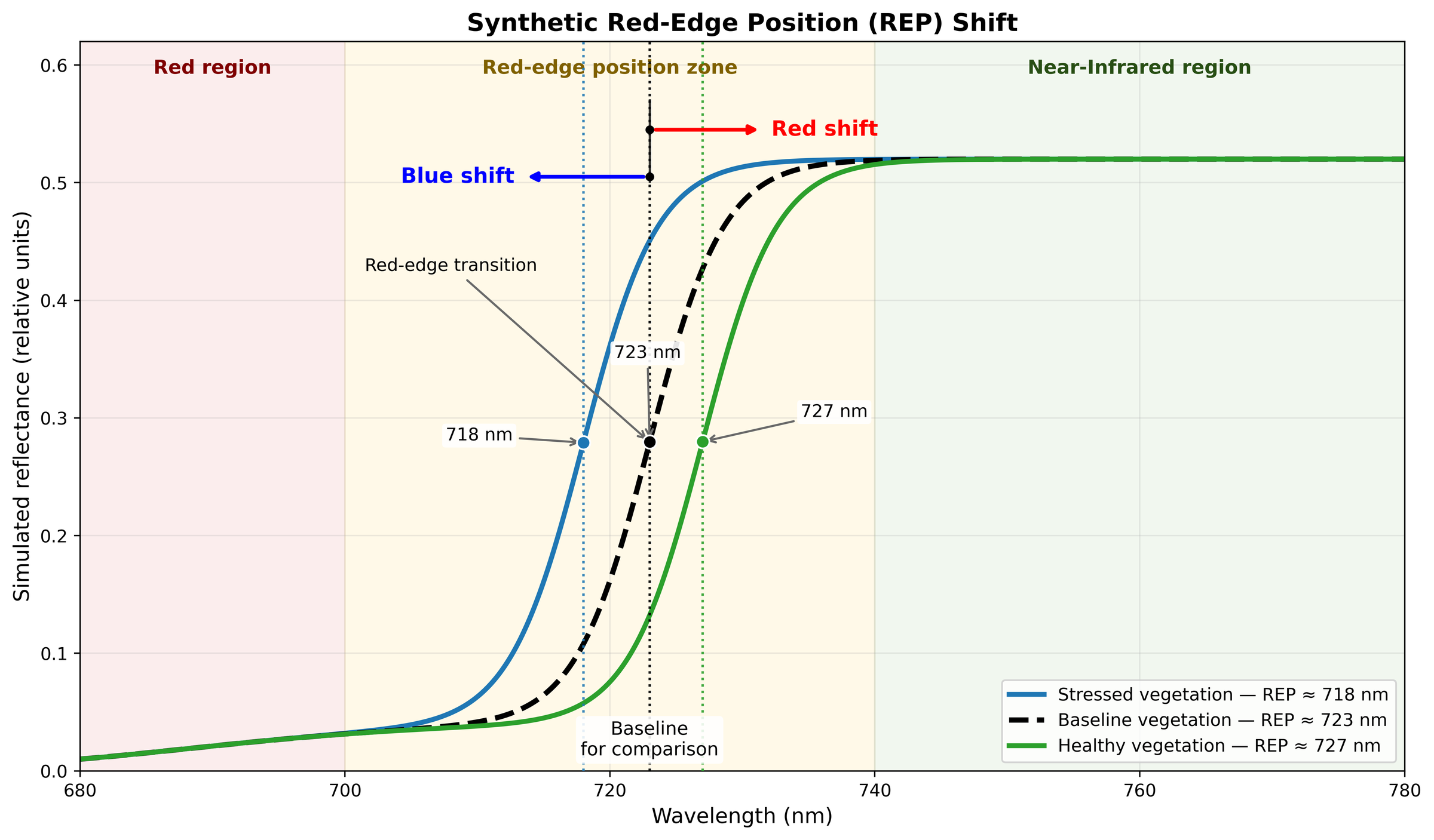
Figure 2:Conceptual illustration of Red-Edge Position (REP) shifts relative to a baseline condition
REP can be calculated in two ways:
(a) Derivative-based REP
REP is defined as the wavelength where the first derivative of reflectance reaches its maximum in the red-edge region:
This definition is especially useful with dense hyperspectral data, as it directly identifies the steepest spectral change.
(b) Four-point interpolation REP
A widely used discrete approximation (Guyot & Baret, 1988):
where reflectance values at 680, 700, 740, and 780 nm are used. The formula estimates the inflection point by linear interpolation between two red-edge anchor bands (700 and 740 nm), using a midpoint target derived from the red and NIR shoulders (680 and 780 nm). This approach requires only four bands, is numerically stable in the presence of sensor noise, and produces results that agree closely with the derivative-based method for Tanager-1’s ~5 nm sampling. Higher REP values indicate stronger chlorophyll content and healthier vegetation; lower values suggest stress or reduced chlorophyll.
Normalized Difference Red Edge (NDRE)
NDRE is a natural progression from NDVI because it replaces the traditional red band with a red-edge band (~720 nm). This substitution makes NDRE more sensitive in dense vegetation, where the red band may saturate. NDRE is especially useful for assessing chlorophyll content in high-biomass canopies. With Tanager-1, you can select the closest available bands or interpolate reflectance to the target wavelengths.
Photochemical Reflectance Index (PRI)
PRI offers a different perspective: it is less about biomass structure and more about photosynthetic function and short-term physiological regulation. PRI is sensitive to the xanthophyll cycle, a mechanism plants use to dissipate excess light energy under stress. Because xanthophyll pigments absorb near 531 nm, PRI can detect rapid physiological changes related to light-use efficiency (LUE) and photosynthetic performance. This highlights a unique capability of hyperspectral data that traditional multispectral vegetation indices cannot easily achieve.
Normalized Difference Water Index (NDWI — vegetation water content, Gao 1996)
NDWI (Gao 1996) measures vegetation liquid water content by leveraging water absorption features in the shortwave infrared (SWIR). Unlike NDVI and EVI, which focus on greenness and chlorophyll, NDWI directly responds to the water present in leaf tissue. This makes it especially valuable for monitoring drought stress, irrigation management, and seasonal water availability. Tanager-1’s spectral range extends into the SWIR, making it well-suited for this analysis.
Note that a different NDWI formulation (McFeeters 1996) is used later in this notebook for water body delineation, which relies on green and NIR bands rather than NIR and SWIR.
Together, these four indices provide complementary information:
REP and NDRE quantify chlorophyll and canopy structure.
PRI assesses real-time photosynthetic efficiency.
NDWI (Gao 1996) evaluates canopy water content.
By combining these indices, you can build a comprehensive biophysical profile of vegetation condition, moving beyond greenness to understand the physiological state of the canopy.
Now that we’ve identified several narrow-band vegetation indices, including how they’re calculated and why they’re useful, it’s time to put this knowledge into action. Now, we’ll use the helper functions we’ve discussed to compute these indices from a real Tanager-1 hyperspectral image. We’ll then visualize and interpret the results, allowing you to see firsthand how these metrics can reveal important information about plant health, canopy structure, and water content.
# Load the vegetation scene, clean the data, and extract specific bands for index calculations.
vegetation_file = "20250501_143138_87_4001_ortho_sr_hdf5.h5"

# load the hs cube with cleanning process
sr_clean_vegetation, attrs, _ = load_hdf5(vegetation_file, clean=True)

wavelengths = attrs['wavelengths']

R_blue  = get_band(sr_clean_vegetation, wavelengths, 475)   # for EVI
R_green = get_band(sr_clean_vegetation, wavelengths, 570)   # for PRI
R_531   = get_band(sr_clean_vegetation, wavelengths, 531)   # for PRI
R_red   = get_band(sr_clean_vegetation, wavelengths, 680)   # for NDVI / EVI
R_700   = get_band(sr_clean_vegetation, wavelengths, 700)   # for REP
R_720   = get_band(sr_clean_vegetation, wavelengths, 720)   # for NDRE
R_740   = get_band(sr_clean_vegetation, wavelengths, 740)   # for REP
R_780   = get_band(sr_clean_vegetation, wavelengths, 780)   # for REP
R_nir   = get_band(sr_clean_vegetation, wavelengths, 800)   # for NDVI / EVI
R_790   = get_band(sr_clean_vegetation, wavelengths, 790)   # for NDRE
R_860   = get_band(sr_clean_vegetation, wavelengths, 860)   # for NDWI
R_1240  = get_band(sr_clean_vegetation, wavelengths, 1240)  # for NDWI
Requested 475 nm -> using 475.98 nm (shift: +0.98 nm)
Requested 570 nm -> using 570.83 nm (shift: +0.83 nm)
Requested 531 nm -> using 530.86 nm (shift: -0.14 nm)
Requested 680 nm -> using 680.89 nm (shift: +0.89 nm)
Requested 700 nm -> using 700.91 nm (shift: +0.91 nm)
Requested 720 nm -> using 720.95 nm (shift: +0.95 nm)
Requested 740 nm -> using 740.98 nm (shift: +0.98 nm)
Requested 780 nm -> using 781.07 nm (shift: +1.07 nm)
Requested 800 nm -> using 801.12 nm (shift: +1.12 nm)
Requested 790 nm -> using 791.09 nm (shift: +1.09 nm)
Requested 860 nm -> using 861.26 nm (shift: +1.26 nm)
Requested 1240 nm -> using 1242.23 nm (shift: +2.23 nm)
Now that we have identified the nearest available bands that will be used to calculate the spectral indices, the next step is to visualize these bands and examine them more closely. Looking at the original reflectance in the selected bands is an important quality-check step, because the reliability of any index depends directly on the quality of the input bands. In practice, if an index appears noisy, the problem often does not come from the index formula itself, but from noise or artifacts already present in one or more of the bands used to compute it. By inspecting the selected bands, we can check the reflectance patterns, evaluate the level of noise, and determine whether unusual index behavior is related to the original spectral data rather than the index calculation. This helps us interpret the results more confidently and identify possible issues such as sensor noise, low signal quality, or artifacts in spectrally sensitive regions.
# Put the selected bands in one place: label -> 2-D reflectance image
selected_bands = {
    "R_blue": R_blue,
    "R_green": R_green,
    "R_531": R_531,
    "R_red": R_red,
    "R_700": R_700,
    "R_720": R_720,
    "R_740": R_740,
    "R_780": R_780,
    "R_nir": R_nir,
    "R_790": R_790,
    "R_860": R_860,
    "R_1240": R_1240,
}

# Figure 1: view each band as an image
fig, axes = plt.subplots(4, 3, figsize=(18, 20), constrained_layout=True)

for ax, (name, image) in zip(axes.ravel(), selected_bands.items()):
    vmin, vmax = contrast_stretching(image)
    im = ax.imshow(image, cmap="gray", vmin=vmin, vmax=vmax)

    ax.set_title(name, fontweight="bold")
    ax.axis("off")
    fig.colorbar(im, ax=ax, shrink=0.75, pad=0.02, label="Reflectance")

fig.suptitle("Band Images Used for Index Calculations", fontweight="bold")
plt.show()

# Figure 2: view each band's pixel-value distribution
fig, axes = plt.subplots(4, 3, figsize=(12, 10), constrained_layout=True)

for ax, (name, image) in zip(axes.ravel(), selected_bands.items()):
    pixels = image[np.isfinite(image)]

    ax.hist(pixels, bins=500, color="black")
    ax.set_title(name, fontweight="bold")
    ax.set_xlabel("Reflectance")
    ax.set_ylabel("Frequency")
    ax.grid(alpha=0.3)

fig.suptitle("Band Pixel Distributions", fontweight="bold")
plt.show()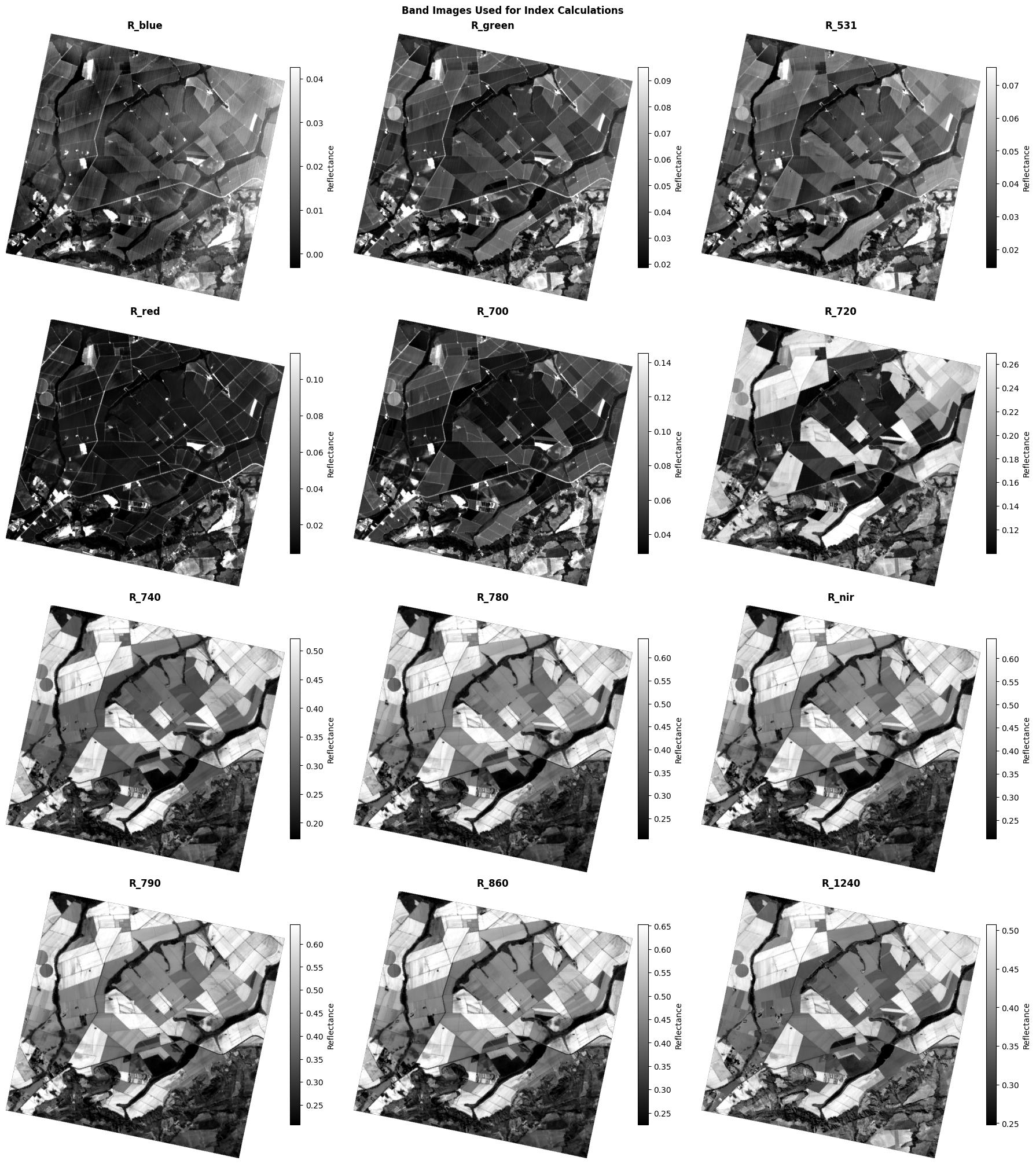
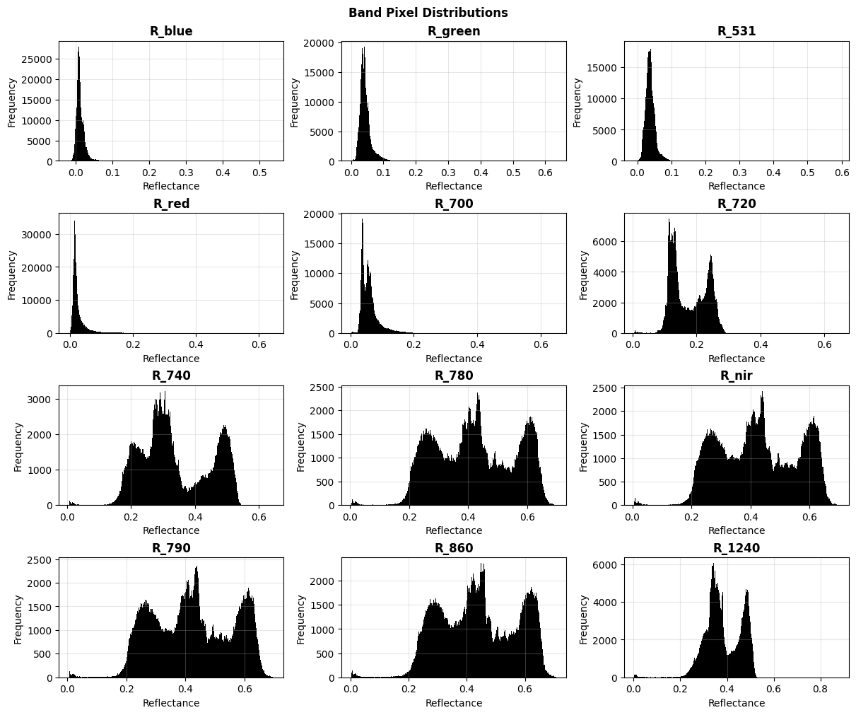
Band visualization: The selected bands show consistent spatial patterns overall, but faint striping artifacts are visible in R_blue, R_green, and R_531. These bands should be interpreted with caution, since such noise can propagate into any narrow-band index derived from them. In contrast, the red-edge and NIR bands (R_720 and beyond) appear cleaner and show less systematic noise, making them more reliable for index calculation.
Histogram interpretation: The histograms confirm that the visible bands (especially R_blue, R_green, and R_531) show low reflectance values concentrated in a narrow range, where noise may have a stronger relative effect on the signal. In the red-edge and NIR regions (R_720 and beyond), the distributions shift toward higher reflectance and show clearer separation between surface types, indicating stronger spectral contrast. Overall, the histograms support the use of the red-edge and NIR bands, while indices involving the visible bands should be interpreted with awareness of potential noise artifacts.
Let’s now calculate the indices and their distributions for interpretation, compare them all, and see what insights we can gain from these together.
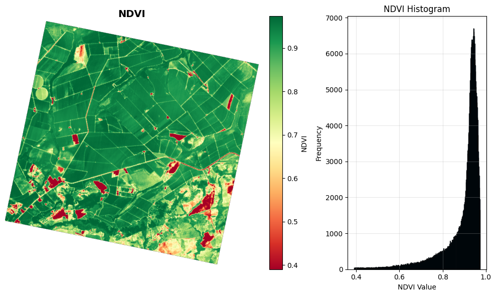
# ---- NDVI (Normalized Difference Vegetation Index) ----
# NDVI compares near-infrared reflectance with red reflectance.
# Healthy vegetation usually reflects strongly in NIR and absorbs strongly in red.
#
# Formula:
# NDVI = (NIR - red) / (NIR + red)

ndvi_numerator = R_nir - R_red
ndvi_denominator = R_nir + R_red

ndvi = safe_divide(ndvi_numerator, ndvi_denominator)
describe_index(ndvi, "NDVI")

plot_index_with_hist(
    ndvi,
    index_name="NDVI",
    hist_label="NDVI Value",
    cmap="RdYlGn",
)
Most NDVI values range from 0.39 to 0.97
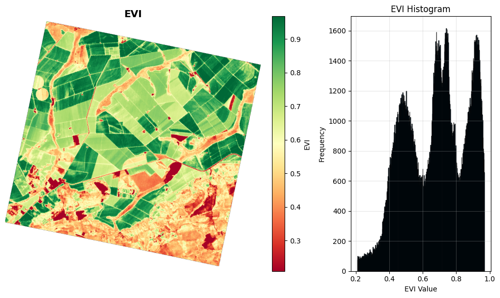
# ---- EVI (Enhanced Vegetation Index) ----
# EVI is similar to NDVI, but it also uses the blue band to reduce atmospheric
# and background effects in dense vegetation.
#
# Formula:
# EVI = gain * (NIR - red) / (NIR + red_weight * red - blue_weight * blue + background)

# Standard EVI constants
# Note: these constants assume reflectance values are unitless, usually between 0 and 1.
gain = 2.5
red_weight = 6.0
blue_weight = 7.5
background = 1.0

evi_numerator = R_nir - R_red
evi_denominator = R_nir + red_weight * R_red - blue_weight * R_blue + background

evi = gain * safe_divide(evi_numerator, evi_denominator)
describe_index(evi, "EVI")

plot_index_with_hist(
    evi,
    index_name="EVI",
    hist_label="EVI Value",
    cmap="RdYlGn",
)
Most EVI values range from 0.21 to 0.97
# ---- REP (Red Edge Position) ----
# REP estimates where the red-edge slope is centered, in nanometers.
# Higher REP values often indicate stronger chlorophyll content.
#
# Formula:
# REP = 700 + 40 * [red_edge_midpoint - R_700] / [R_740 - R_700]

red_edge_midpoint = (R_red + R_780) / 2.0
rep_numerator = red_edge_midpoint - R_700
rep_denominator = R_740 - R_700

rep = 700.0 + 40.0 * safe_divide(rep_numerator, rep_denominator)
describe_index(rep, "REP", units="nm")

plot_index_with_hist(
    rep,
    index_name="REP (Red Edge Position)",
    hist_label="REP Value (nm)",
    cmap="magma",
)
Most REP values range from 717.39 nm to 728.80 nm
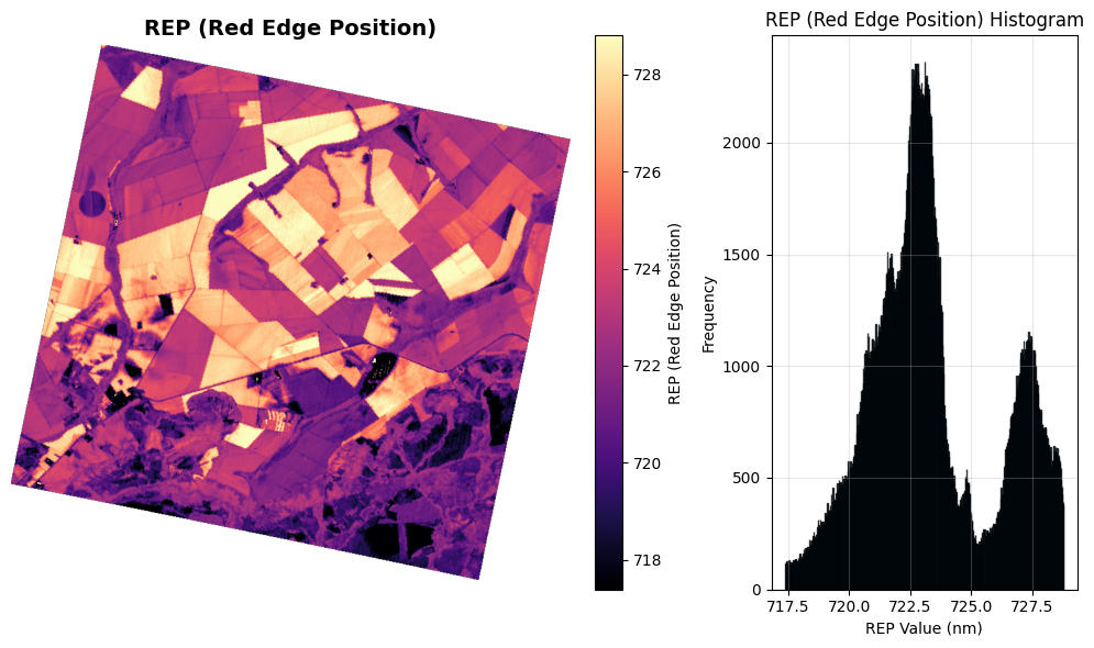
The REP map shows that, unlike standard vegetation indices that calculate dimensionless ratios, the Red Edge Position identifies a physical wavelength on the electromagnetic spectrum. While we utilized the four-point interpolation method to estimate REP across the spatial map above, the underlying physical shift is driven primarily by chlorophyll concentration and overall plant stress. To understand the exact mechanics of this shift, we will analyze the spectral signatures of fields 1 (F-1) and 6 (F-6) presented in Figure 3. For this detailed field-level analysis, we employ the derivative method to precisely isolate the inflection point, as these two fields appear to share similar canopy structure but exhibit distinct chlorophyll differences.
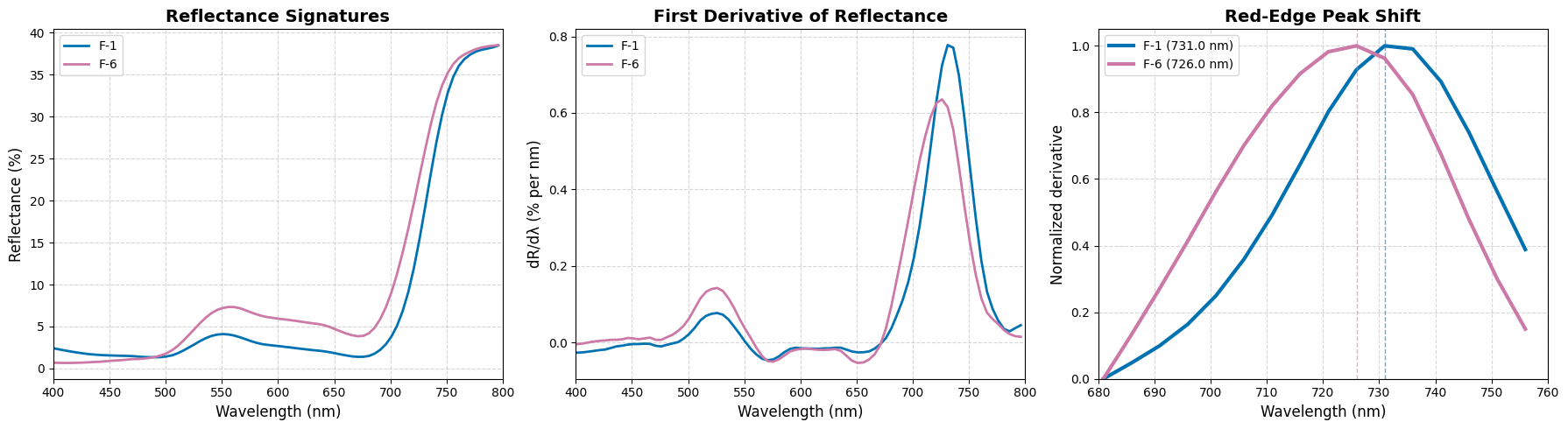
Figure 3:Derivative-based red-edge analysis comparing fields with different chlorophyll content
The derivative-based spectral analysis for these two fields reveals critical differences in canopy biophysics and plant health:
Reflectance Signatures (Left Panel): F-6 exhibits a marked increase in visible light reflectance, specifically within the red absorption well (~650–680 nm) and the green peak (~550 nm). Because healthy, photosynthetically active canopies strongly absorb red light, this elevated reflectance in F-6 directly indicates a significant reduction in chlorophyll concentration compared to the vigorous F-1 canopy.
First Derivative of Reflectance (Middle Panel): By computing the first derivative of the reflectance spectra (), we isolate the exact inflection point of the red edge—the abrupt transition between red chlorophyll absorption and near-infrared (NIR) structural reflectance. F-1 displays a sharper, higher-amplitude peak, which is characteristic of dense, healthy biomass with high photosynthetic capacity.
Red-Edge Peak Shift (Right Panel): This normalized view explicitly isolates the Red Edge Position (REP). The healthy F-1 canopy peaks at 731.0 nm. In contrast, the lower chlorophyll content in F-6 narrows its red absorption feature, forcing the inflection point to retreat toward shorter wavelengths, resulting in a pronounced “blue shift” to 726.0 nm. This quantifiable 5.0 nm shift serves as a precise hyperspectral indicator of physiological stress or early senescence in F-6.
Based on this field-level analysis and the observed spectral shifts, we can interpret the REP map with appropriate caution. As REP increases (red shift), this indicates a higher concentration of canopy chlorophyll, which typically correlates with robust nitrogen uptake, denser biomass, or vigorous vegetative growth.
When we scale this understanding back to the spatial map, we can categorize the landscape into distinct biophysical zones:
Strong Red Shift (Light Yellow/White, > 726 nm): These fields represent peak biophysical conditions for this region. The canopies here are exceptionally dense and packed with chlorophyll, aligning with the vigorous F-1 signature analyzed above.
Baseline/Moderate Shift (Pink/Orange, ~722–724 nm): This represents the intermediate state for the majority of vegetated surfaces in this scene. These are likely fields in a different phenological stage or crop species with naturally lower chlorophyll density.
Strong Blue Shift (Dark Purple/Black, < 718 nm): These areas represent severe reduction or total absence of active chlorophyll, corresponding to bare soil, non-agricultural infrastructure, or crops that have fully senesced prior to harvest.
Finally, the accompanying histogram statistically validates what we observe spatially. The stark bimodal (two-peak) distribution confirms that vegetation in this landscape is distinctly divided into two primary biophysical states. The dominant primary peak around 722.5 nm captures the widespread, moderately vigorous baseline crops, while the secondary peak near 727.5 nm isolates the subset of highly vigorous, red-shifted fields. By coupling the map with the histogram, we can quantitatively group these fields by their physiological maturity and nutrient status, extracting meaningful insights even without prior ground-truth knowledge of the specific crop types planted.
# ---- NDRE (Normalized Difference Red Edge) ----
# NDRE is similar to NDVI, but it uses a red-edge band instead of the red band.
# This helps keep sensitivity in dense vegetation where NDVI can saturate.
#
# Formula:
# NDRE = (R_790 - R_720) / (R_790 + R_720)

ndre_numerator = R_790 - R_720
ndre_denominator = R_790 + R_720

ndre = safe_divide(ndre_numerator, ndre_denominator)
describe_index(ndre, "NDRE")

plot_index_with_hist(
    ndre,
    index_name="NDRE (Normalized Difference Red Edge)",
    hist_label="NDRE Value",
    cmap="BrBG",
)
Most NDRE values range from 0.14 to 0.59
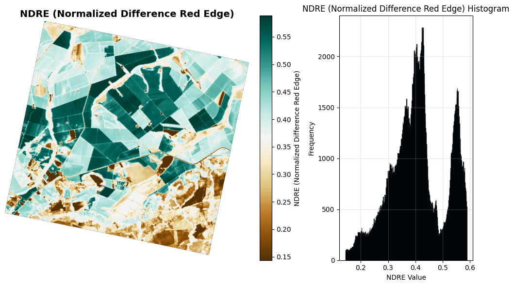
Having characterized the biophysical groupings extracted from the Red Edge Position (REP) analysis, we can now use the NDRE map to validate those findings. While REP measures the physical wavelength of the red edge shift, NDRE measures the relative amplitude of reflectance using a narrow band situated directly on that slope Delegido et al., 2013.
Crucially, the NDRE results should mathematically and spatially follow the pattern of the REP map: as a canopy accumulates chlorophyll, the red edge shifts to longer wavelengths (higher REP), which simultaneously increases the resulting NDRE value.
Observing the NDRE map, we see values ranging from approximately 0.05 to 0.19. The spatial patterns act as a direct validation of our REP analysis:
Dark Teal (High values, > 0.16): These fields exhibit the highest chlorophyll concentrations and canopy densities in the scene. Spatially, these align precisely with the “bright yellow” fields from the REP map that exhibited the strongest red shift.
White/Light Teal (Moderate values, ~0.10–0.14): This represents the baseline chlorophyll state for the majority of vegetated surfaces. These areas correspond exactly with the moderate “pink/orange” zones in the REP map.
Brown (Low values, < 0.09): These areas represent non-photosynthetic surfaces (bare soil, infrastructure, or fully senesced vegetation), closely matching the “blue-shifted” dark purple areas in the previous analysis.
The NDRE histogram provides statistical confirmation of this correlation. Just like the REP histogram, the NDRE data exhibits a pronounced bimodal (two-peak) distribution, confirming that the landscape is clearly partitioned into two dominant biophysical states:
The Primary Peak (~0.10–0.11): This massive central cluster captures the widespread, moderately vigorous baseline crops.
The Secondary Peak (~0.17–0.18): This distinct peak isolates the sub-population of highly vigorous, high-chlorophyll fields.
The strong correspondence between NDRE amplitude and REP wavelength shift provides independent confirmation of the spatial patterns we observe. Using two distinct mathematical approaches—one measuring wavelength position, the other measuring reflectance amplitude—we consistently identify the same biophysical groupings across the landscape. This suggests that the observed variation in chlorophyll content represents genuine differences in crop condition or management, rather than noise or artifacts, though field validation would be needed to determine the specific causes (such as crop species, planting dates, or nitrogen application rates).
# ---- PRI (Photochemical Reflectance Index) ----
# PRI compares reflectance near 531 nm with green reflectance near 570 nm.
# It is often used as a relative indicator of photosynthetic light-use efficiency.
#
# Formula:
# PRI = (R_531 - R_green) / (R_531 + R_green)

pri_numerator = R_531 - R_green
pri_denominator = R_531 + R_green

pri = safe_divide(pri_numerator, pri_denominator)
describe_index(pri, "PRI")

plot_index_with_hist(
    pri,
    index_name="PRI (Photochemical Reflectance Index)",
    hist_label="PRI Value",
    cmap="RdYlBu",
)
Most PRI values range from -0.19 to 0.00
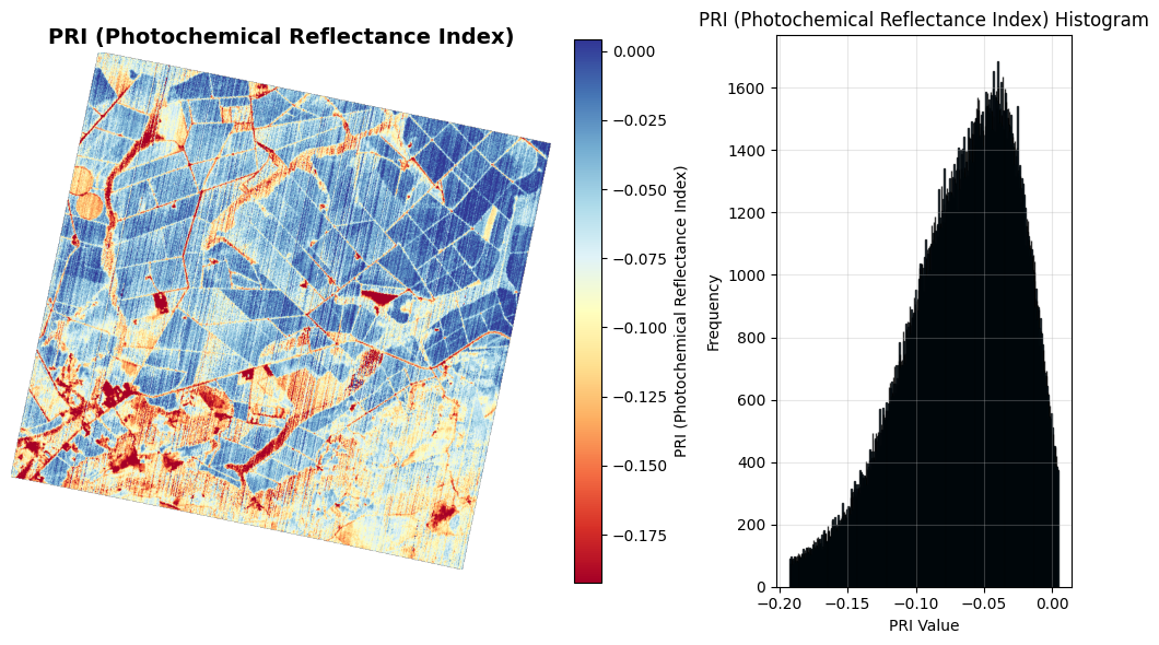
While our previous indices (REP and NDRE) quantified the capacity of the canopy—specifically its structural density and total chlorophyll concentration—the Photochemical Reflectance Index (PRI) Gamon et al., 2012 was originally designed to track the operational efficiency of photosynthesis at the leaf level. PRI is sensitive to the xanthophyll cycle, a rapid photoprotective mechanism that helps plants dissipate excess light energy.
However, applying PRI at the canopy scale introduces important complications that we must acknowledge.
From Leaf to Canopy: What Changes
At the leaf level, PRI responds to short-term (minutes to hours) changes in the xanthophyll cycle, providing a direct measure of photosynthetic light-use efficiency. At the canopy scale from satellite imagery like Tanager-1, the signal becomes more complex:
Structural interference: Canopy density (LAI), architecture, and the ratio of sunlit to shaded leaves can dominate the PRI signal, sometimes overwhelming the physiological component.
Background contamination: Soil reflectance, non-photosynthetic vegetation (stems, litter), and canopy gaps contribute to the measured signal.
Viewing geometry: Shadow fractions and sun-sensor geometry can significantly alter PRI values independent of plant physiology.
Temporal meaning shifts: Rather than tracking instantaneous xanthophyll dynamics, canopy-scale PRI often reflects longer-term pigment pool composition (the ratio of carotenoids to chlorophyll accumulated over weeks).
Because of these factors, canopy-scale PRI should be interpreted cautiously as a relative indicator of vegetation condition rather than a direct measure of instantaneous photosynthetic efficiency.
Interpreting the PRI Map
Looking at the spatial distribution, the values range from approximately -0.20 to 0.00:
Dark Blue (Higher values, near 0.00 to -0.05): These regions may indicate vegetation with favorable pigment ratios and canopy structure. However, without ground truth, we cannot determine whether this reflects true photosynthetic efficiency, higher LAI, or differences in canopy architecture.
Light Blue/Yellow (Moderate values, ~ -0.07 to -0.12): These intermediate values could reflect various conditions: different crop species with naturally different pigment compositions, varying canopy densities, or actual differences in stress response.
Red/Dark Red (Low values, < -0.15): These areas correspond to non-photosynthetic surfaces (bare soil, roads) or fully senescent vegetation.
The PRI Histogram: A Different Pattern
The PRI histogram reveals an important contrast with our earlier analyses. Unlike the starkly bimodal (two-peak) distributions we observed for chlorophyll content (REP and NDRE), the PRI histogram is overwhelmingly unimodal (single peak):
The Dominant Peak (~ -0.05): The vast majority of pixels cluster tightly around this value.
The Long Left Tail: A gradual transition into non-vegetated or senescent surfaces.
What Does This Tell Us?
This unimodal distribution suggests that despite the two distinct tiers of chlorophyll density we identified earlier, the fields share relatively similar PRI values. This pattern is consistent with several possible interpretations:
Similar pigment pool ratios: The different crop types may maintain comparable carotenoid-to-chlorophyll ratios despite having different total chlorophyll concentrations.
Structural compensation: Lower-chlorophyll crops might have canopy architectures that produce similar PRI signals to denser crops.
Comparable stress levels: If PRI is responding to stress at this scale, the relatively narrow distribution suggests that stress levels are fairly uniform across the agricultural landscape.
Important Limitations
Without ground truth data (crop species, growth stage, LAI measurements, or direct photosynthetic measurements), we cannot definitively attribute the PRI patterns to any single factor. Canopy-scale PRI is best used as a relative comparative tool within a scene or time series, rather than as an absolute measure of photosynthetic function. To validate physiological interpretations, PRI should ideally be:
Combined with structural indices (NDVI, EVI) to separate biomass effects
Calibrated against field measurements of actual photosynthetic rates or pigment concentrations
Interpreted alongside environmental data (temperature, moisture, time of day)
Analyzed as part of a time series to track changes rather than relying on single-date snapshots
# ---- NDWI (Gao 1996 vegetation water index) ----
# This NDWI version compares NIR and SWIR reflectance to estimate vegetation water content.
# It is different from the open-water NDWI used later in the notebook.
#
# Formula:
# NDWI = (R_860 - R_1240) / (R_860 + R_1240)

ndwi_numerator = R_860 - R_1240
ndwi_denominator = R_860 + R_1240

ndwi = safe_divide(ndwi_numerator, ndwi_denominator)
describe_index(ndwi, "NDWI (vegetation water)")

plot_index_with_hist(
    ndwi,
    index_name="NDWI (Gao 1996 Water Index)",
    hist_label="NDWI Value",
    cmap="Blues",
)
Most NDWI (vegetation water) values range from -0.14 to 0.16
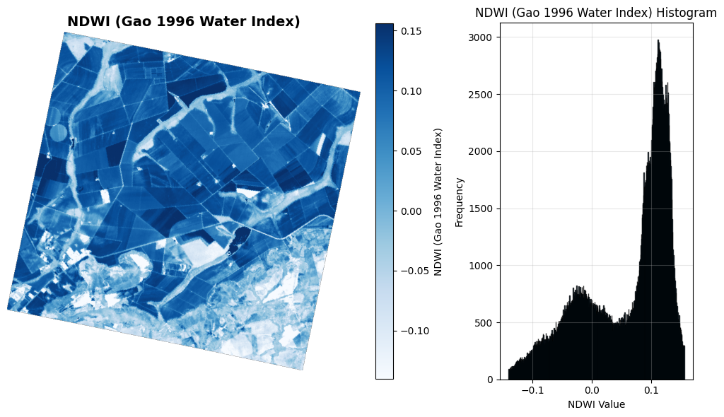
Having established the chlorophyll concentration (REP, NDRE) and the operational efficiency (PRI) of the vegetation in this scene, we now turn to the Normalized Difference Water Index (NDWI) Gao, 1996 to evaluate the physical hydration of the canopy. Because NDWI utilizes the shortwave infrared (SWIR) region—which is highly sensitive to liquid water molecule absorption—it provides a direct biophysical proxy for the Equivalent Water Thickness (EWT) within the leaf cellular structure.
The spatial distribution of NDWI values ranges from approximately -0.15 to 0.15. By analyzing this spatial heterogeneity, we can map the canopy moisture profile across the landscape:
Dark Blue (High values, > 0.08): These fields contain the highest volume of liquid water within their canopies. Spatially, these areas encompass almost all of the vegetated fields we identified previously, including both the “super-green” (highly red-shifted) and the baseline/moderate chlorophyll fields.
Light Blue/White (Low values, < 0.00): These areas represent surfaces with minimal to no liquid water content. These precisely mirror the spatial footprint of the bare soil, roads, and fully senesced, dry vegetation identified in the previous maps.
The NDWI histogram provides crucial statistical context for the entire scene, displaying a clear bimodal distribution:
The Dominant Right Peak (~0.10 - 0.15): The vast majority of the pixels form a massive, high-value peak. This statistically confirms that the bulk of the agricultural landscape is maintaining a high internal water content.
The Left Peak/Shoulder (~ -0.05 to 0.00): This smaller grouping captures the dry, non-vegetated background surfaces and infrastructure.
The NDWI analysis provides important environmental context for interpreting this landscape.
Earlier, the REP and NDRE maps revealed that the crops were split into two distinct tiers of chlorophyll concentration (high vs. moderate). The NDWI map now shows that both tiers share similarly high canopy moisture levels (the massive right-hand peak). Combined with the relatively uniform PRI distribution observed earlier, this suggests that water availability appears adequate across the agricultural landscape.
By integrating these hyperspectral observations, we can infer that the moderate-chlorophyll fields are unlikely to be experiencing severe drought stress. The combination of high water content (NDWI) and relatively similar pigment ratios (PRI) across both chlorophyll tiers suggests that the spatial variations in chlorophyll (REP/NDRE) may be driven by factors other than water limitation—such as natural phenological differences (e.g., different planting dates or crop species) or variable nitrogen management. However, definitive attribution would require ground truth validation.
Conclusion
By integrating multiple spectral indices into our workflow, we move beyond simply measuring “greenness” to building a more comprehensive biophysical profile of the agricultural landscape. Each index alone provides a limited perspective; it is through their combined interpretation that we can begin to disentangle factors such as canopy structure, biochemical properties, and physiological condition. This multi-index approach enables richer insights than any single index could offer.
Interpreting the Multi-Index Profile
Based on the combined observations from six spectral indices, several patterns emerge:
Chlorophyll variation (REP, NDRE): The landscape shows two distinct tiers of chlorophyll concentration, indicating structural or developmental differences between fields.
Water status (NDWI): Both chlorophyll tiers maintain similarly high canopy moisture levels, suggesting adequate water availability across most of the scene.
Pigment ratios (PRI): The relatively uniform PRI distribution suggests comparable carotenoid-to-chlorophyll ratios across the landscape, though interpretation at canopy scale requires caution.
What This Suggests
The combination of high water content, robust chlorophyll levels in many fields, and relatively uniform pigment ratios is consistent with a vigorous agricultural landscape during active growing season. The observed chlorophyll variations appear more likely related to crop type, planting schedules, or nutrient management than to water stress or disease, given the high moisture levels throughout.
However, without ground truth data on crop species, growth stages, management practices, or field measurements, these interpretations remain inference rather than confirmation. The true value of this multi-index workflow lies not in providing definitive answers, but in generating testable hypotheses about landscape condition that can guide targeted field validation and monitoring strategies.
Ultimately, this workflow demonstrates that strategically combining narrow-band indices allows us to develop multi-dimensional vegetation profiles that reveal spatial patterns and suggest potential drivers—moving beyond basic monitoring toward hypothesis-driven investigation of agricultural landscapes.
Application: Water Body Masking and Quality Analysis
In this section, we explore a targeted workflow using the water-focused Tanager-1 scene: 20250504_025815_32_4001_ortho_sr_hdf5.h5.
Hyperspectral imagery’s narrow, contiguous spectral bands enable precise targeting of specific absorption features. This capability is particularly valuable for water quality assessments, where spectral features such as chlorophyll absorption can be subtle and easily obscured by broader spectral bands.
To analyze the water bodies in this scene, we will calculate two specific narrow-band indices:
NDWI (Normalized Difference Water Index): Used to delineate open water features. By exploiting the strong absorption of water in the near-infrared (NIR) and its relative reflectance in the green band, we can effectively isolate water from surrounding land and vegetation.
NDCI (Normalized Difference Chlorophyll Index): Designed to estimate chlorophyll-a concentrations, which can serve as a proxy for algal biomass and potential indicators of eutrophication or water quality changes. It specifically targets the red edge and red reflectance peaks.
The Two-Step Pipeline
Applying a biochemical index like NDCI across an entire unmasked scene often results in noisy or misleading values, as terrestrial vegetation also contains chlorophyll. To prevent this, we will implement a practical, two-step masking workflow:
Delineation: Compute the NDWI across the entire scene to generate a binary mask, separating water pixels from land.
Targeted Assessment: Apply the NDCI calculation strictly within the boundaries of the water mask.
By applying this sequence, we ensure that we focus our aquatic chlorophyll concentration calculation on the relevant image pixels.
# Load the water-body scene and extract its wavelength metadata.
sr_clean_water, water_attrs, _ = load_hdf5(water_sr_path, clean=True)
wavelengths_water = water_attrs["wavelengths"]
# Select the bands needed for the water-body indices.
R_green_water = get_band(sr_clean_water, wavelengths_water, 560) # green band for open-water NDWI
R_red_water = get_band(sr_clean_water, wavelengths_water, 665) # red band for NDCI
R_red_edge_water = get_band(sr_clean_water, wavelengths_water, 705) # red-edge band for NDCI
R_nir_water = get_band(sr_clean_water, wavelengths_water, 842) # NIR band for open-water NDWI
# ---- NDWI (McFeeters 1996 open-water index) ----
# Formula: NDWI = (green - NIR) / (green + NIR)
ndwi_water_numerator = R_green_water - R_nir_water
ndwi_water_denominator = R_green_water + R_nir_water
ndwi_water = safe_divide(ndwi_water_numerator, ndwi_water_denominator)
describe_index(ndwi_water, "NDWI (open water)")
# ---- NDCI (Normalized Difference Chlorophyll Index) ----
# Formula: NDCI = (red edge - red) / (red edge + red)
ndci_numerator = R_red_edge_water - R_red_water
ndci_denominator = R_red_edge_water + R_red_water
ndci = safe_divide(ndci_numerator, ndci_denominator)
describe_index(ndci, "NDCI")Requested 560 nm -> using 560.83 nm (shift: +0.83 nm)
Requested 665 nm -> using 665.87 nm (shift: +0.87 nm)
Requested 705 nm -> using 705.92 nm (shift: +0.92 nm)
Requested 842 nm -> using 841.21 nm (shift: -0.79 nm)
Most NDWI (open water) values range from -0.69 to 0.43
Most NDCI values range from -0.07 to 0.58
# Use NDWI to keep only likely open-water pixels before interpreting NDCI.
# Positive NDWI values generally indicate open water in this formulation.
water_pixels = ndwi_water > 0
ndci_water_only = np.where(water_pixels, ndci, np.nan)

describe_index(ndci_water_only, "NDCI over water pixels")

plot_index_with_hist(
    ndwi_water,
    index_name="NDWI - Open Water (McFeeters 1996)",
    hist_label="NDWI Water Value",
    cmap="Blues",
)

plot_index_with_hist(
    ndci_water_only,
    index_name="NDCI - Water Chlorophyll (water pixels only)",
    hist_label="NDCI Value",
    cmap="viridis",
    vmin=-0.1,
    vmax=0.5,
)
Most NDCI over water pixels values range from -0.08 to 0.10
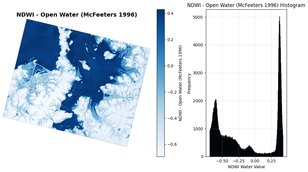
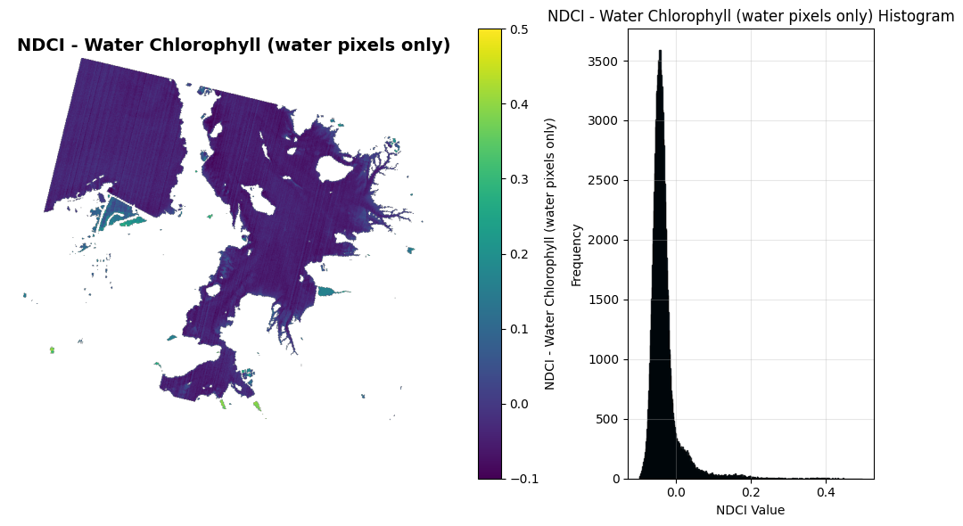
As you can see, this workflow works successfully, the NDWI map effectively isolates the hydrological features in the scene. Water bodies are distinctly highlighted in dark blue (representing higher index values), while the surrounding land and vegetation appear in lighter blues and white. By leveraging the bimodal distribution of these NDWI values, we can confidently threshold the data to establish a robust binary water mask. With the land effectively removed, we apply the NDCI calculation strictly within the confirmed water pixels. This step highlights chlorophyll-a concentrations, serving as a proxy for algal biomass, potential eutrophication, and overall water health. Looking closely at the resulting NDCI map, you can now clearly identify localized hotspots where values exceed 0.2 (visible as the green and yellow pixels). These elevated values are strong indicators of active algal blooms or areas experiencing significant nutrient loading, allowing us to pinpoint locations where water quality concerns may be immediately relevant.
If we had applied the NDCI across the entire unmasked scene, the chlorophyll content in terrestrial vegetation would have heavily skewed the results. By establishing a binary mask first, we focus only on relevant pixels, allowing for a precise, targeted assessment of chlorophyll concentration within the water system itself.
Lesson Summary
Across both scenes, this lesson demonstrated that narrow-band spectral indices unlock capabilities that broadband multispectral data cannot match:
Vegetation scene (Brazil): REP and NDRE revealed two distinct tiers of chlorophyll concentration; NDWI confirmed high canopy moisture across both tiers; PRI pointed to comparable pigment ratios, suggesting the variation is driven by crop type or phenology rather than water stress.
Water body scene (South Korea): NDWI (McFeeters 1996) produced a clean binary water mask, and NDCI — applied only within confirmed water pixels — identified localised chlorophyll-a hotspots consistent with algal bloom activity.
The key takeaway is that no single index answers every question. Combining structurally focused indices (REP, NDRE), physiologically focused indices (PRI), water-content indices (NDWI-veg), and water-body indices (NDWI-water, NDCI) into a multi-index workflow produces interpretations that are far richer and more defensible than any single metric alone.
What’s next?
In this lesson, we used spectral indices to turn carefully selected bands into meaningful measurements: greenness, red-edge position, photosynthetic behavior, vegetation water content, open-water extent, and water chlorophyll indicators. This is a powerful way to use hyperspectral data when we already know which wavelengths are important for a specific question.
But hyperspectral data contains far more information than the handful of bands used in any single index. A Tanager-1 cube includes hundreds of narrow, contiguous bands, and many of them carry overlapping but useful information. This leads to a natural next question:
Can we summarize the full hyperspectral cube without choosing only a few bands by hand?
In the next lesson, Dimensionality Reduction: Principal Component Analysis (PCA), we will move from index-based analysis to full-cube analysis. Instead of calculating one index at a time, we will use PCA to compress many spectral bands into a smaller number of components that preserve the strongest patterns in the data. This helps us visualize high-dimensional hyperspectral imagery, reduce redundancy between bands, and prepare spectral data for more advanced analysis and machine learning workflows.
So the progression is:
Spectral indices: use expert-selected wavelengths to answer targeted questions.
Dimensionality reduction: use the full spectral cube to discover broad patterns across all bands.
Continue to module_4/02_Dim_Reduction.ipynb to see how PCA helps us work with the full hyperspectral dataset.
- Delegido, J., Verrelst, J., Meza, C. M., Rivera, J. P., Alonso, L., & Moreno, J. (2013). A red-edge spectral index for remote sensing estimation of green LAI over agroecosystems. International Journal of Applied Earth Observation and Geoinformation, 24, 42–52.
- Gamon, J. A., Peñuelas, J., & Field, C. B. (2012). A narrow-waveband spectral index that tracks diurnal changes in photosynthetic efficiency. New Phytologist. 10.1111/j.1469-8137.2011.03791.x
- Gao, B.-C. (1996). NDWI—A normalized difference water index for remote sensing of vegetation liquid water from space. Remote Sensing of Environment, 58(3), 257–266.
- McFeeters, S. K. (1996). The use of the Normalized Difference Water Index (NDWI) in the delineation of open water features. International Journal of Remote Sensing, 17(7), 1425–1432. 10.1080/01431169608948714