Welcome to Lesson 2 of Module 3.
This lesson serves as a bridge to the most exciting part of our hyperspectral data analysis course for Tanager.
Up to this point, our focus has been on building a solid foundation in understanding, accessing, and preprocessing data. You now have an analysis-ready hyperspectral cube. Now it is time to transition from raw pixels to actionable insights by implementing advanced analytical techniques and machine learning.
Figure 1 shows how the workflow typically begins once you have an analysis-ready hyperspectral cube. Depending on your objective, you may begin by calculating spectral indices, classifying land cover, or applying regression models to estimate biophysical variables, each of which produces different map outputs.
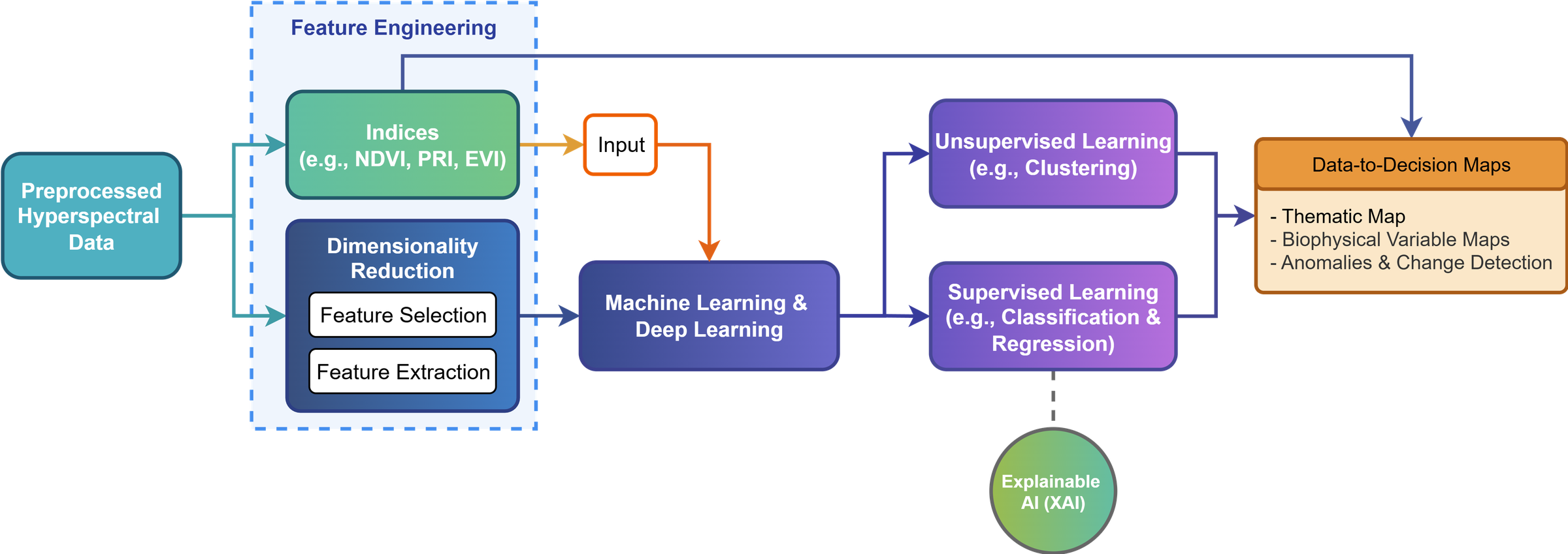
Figure 1:A comprehensive data-to-decision framework for hyperspectral remote sensing.
As shown in Figure 1, the hyperspectral data workflow is organized as an interconnected sequence of steps, beginning with preprocessed hyperspectral data and progressing through feature engineering, machine learning, and map generation. In this course, we are going to cover this workflow step by step, explaining how each stage contributes to transforming hyperspectral data into meaningful map products for analysis and decision-making.
Before we explore each step in detail, it is helpful to break down the main concepts in this workflow and define what each one means in the context of hyperspectral remote sensing.
Feature Engineering
Feature engineering in hyperspectral remote sensing involves transforming high-dimensional spectral measurements into more informative variables that enhance data interpretation, improve class separability, and increase the performance of statistical and machine learning models. In this study, feature engineering is considered in two main forms: spectral index calculation and dimension reduction. As shown in Figure 2, the workflow begins with the hyperspectral data cube and proceeds through feature engineering operations that either derive spectral indices or reduce spectral dimensionality through feature selection and feature extraction.
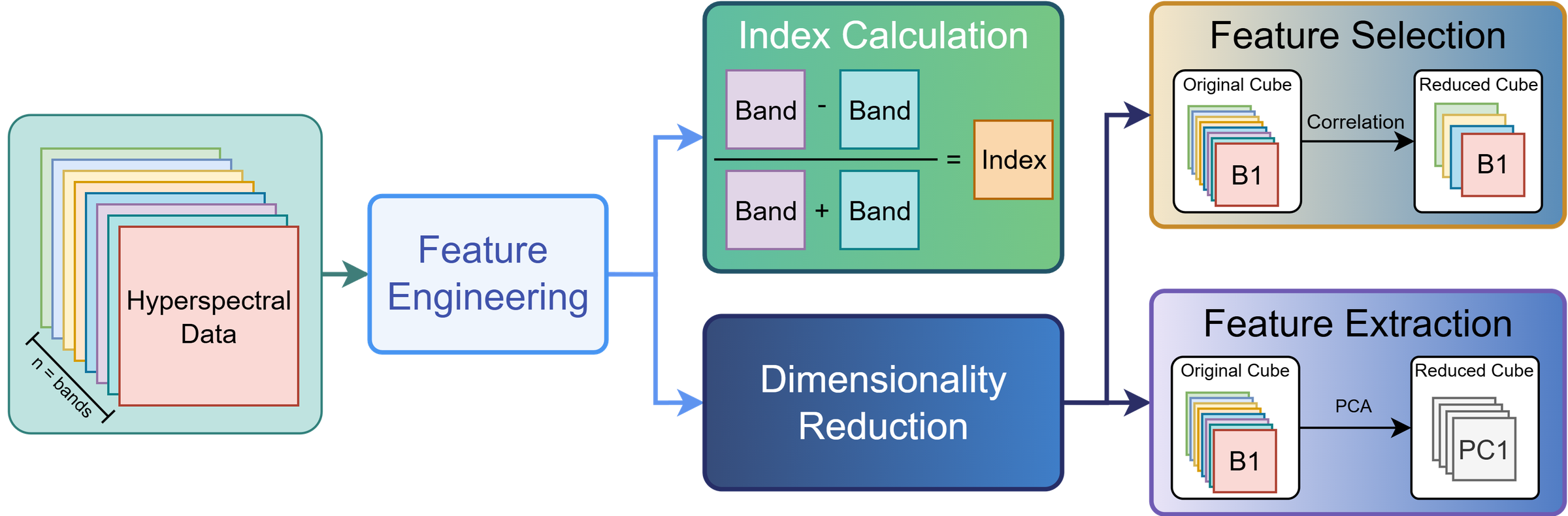
Figure 2:Feature engineering workflow for hyperspectral data analysis.
Spectral Index Calculation
Spectral indices are derived by combining reflectance values from selected wavelength bands to emphasize specific biophysical or biochemical surface properties. Common examples include the Normalized Difference Vegetation Index (NDVI), the Photochemical Reflectance Index (PRI), and the Enhanced Vegetation Index (EVI). These indices are designed to amplify diagnostically relevant spectral responses, making them particularly useful for applications such as vegetation monitoring, stress detection, and surface condition assessment, as illustrated in Figure 3.
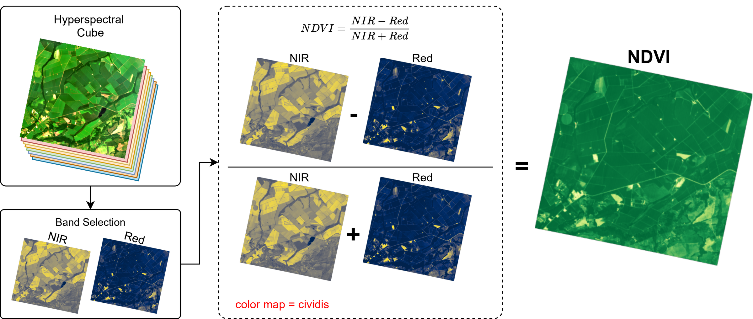
Figure 3:Spectral Index Calculation (e.g., NDVI)
Dimensionality Reduction
Hyperspectral datasets typically contain hundreds of contiguous bands, many of which are highly correlated and may also include redundant or noisy information. Dimensionality reduction addresses this challenge by reducing data complexity while preserving the most meaningful spectral information. This can be achieved through feature selection, which identifies and retains the most relevant original bands, or through feature extraction, which transforms the original data into a reduced set of new variables, such as principal components analysis (PCA). These approaches improve computational efficiency, can reduce the risk of overfitting, and facilitate more robust downstream analysis, as illustrated in Figure 4.
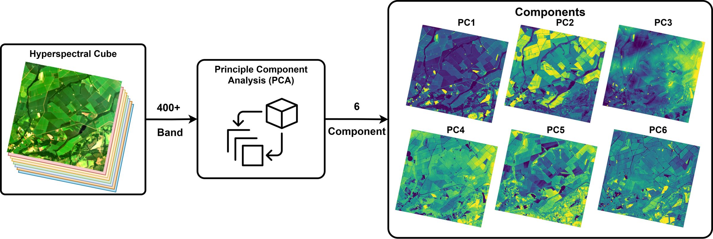
Figure 4:Dimensionality Reduction (e.g., Principal Component Analysis)
Machine Learning (ML)
Machine learning is the process of training algorithms to detect patterns, relationships, or structures in data and use them to make predictions or group similar observations. In hyperspectral remote sensing, machine learning is especially valuable because the data are often high-dimensional and complex, making traditional manual interpretation difficult.
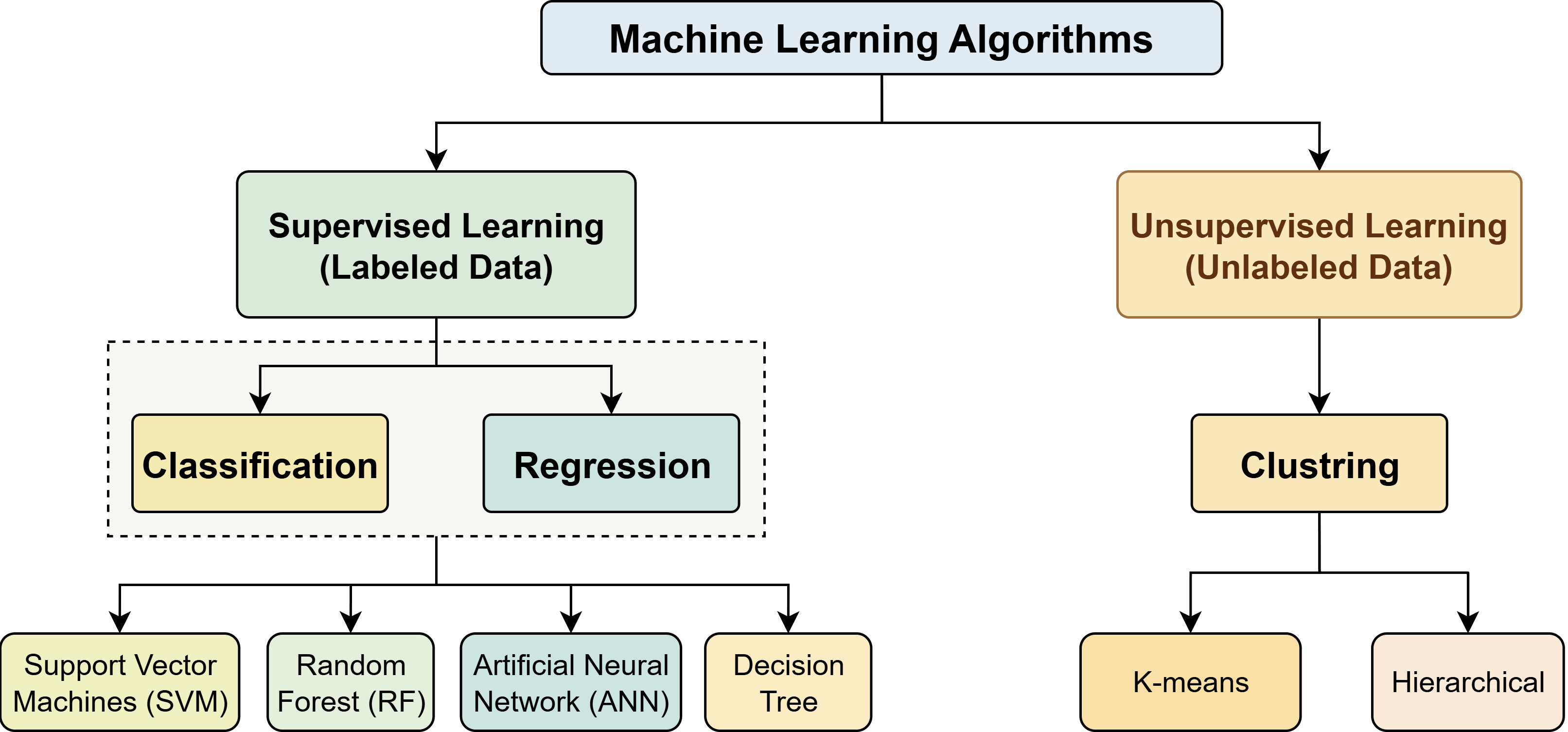
Figure 5:Diagram showing the three main types of machine learning algorithms: supervised, unsupervised, and reinforcement learning
As shown in Figure 5, machine learning methods are commonly divided into supervised and unsupervised approaches. In supervised learning, the model is trained using labeled data, meaning that the correct class or target value is already known for a set of samples. These methods are widely used for tasks such as land-cover classification and regression-based estimation of biophysical variables. In unsupervised learning, the model works with unlabeled data and identifies natural patterns or groupings on its own. This is useful for tasks such as clustering, anomaly detection, and exploratory analysis when reference data are limited or unavailable. The difference between labled and unlabled datasets is shown in Figure 6
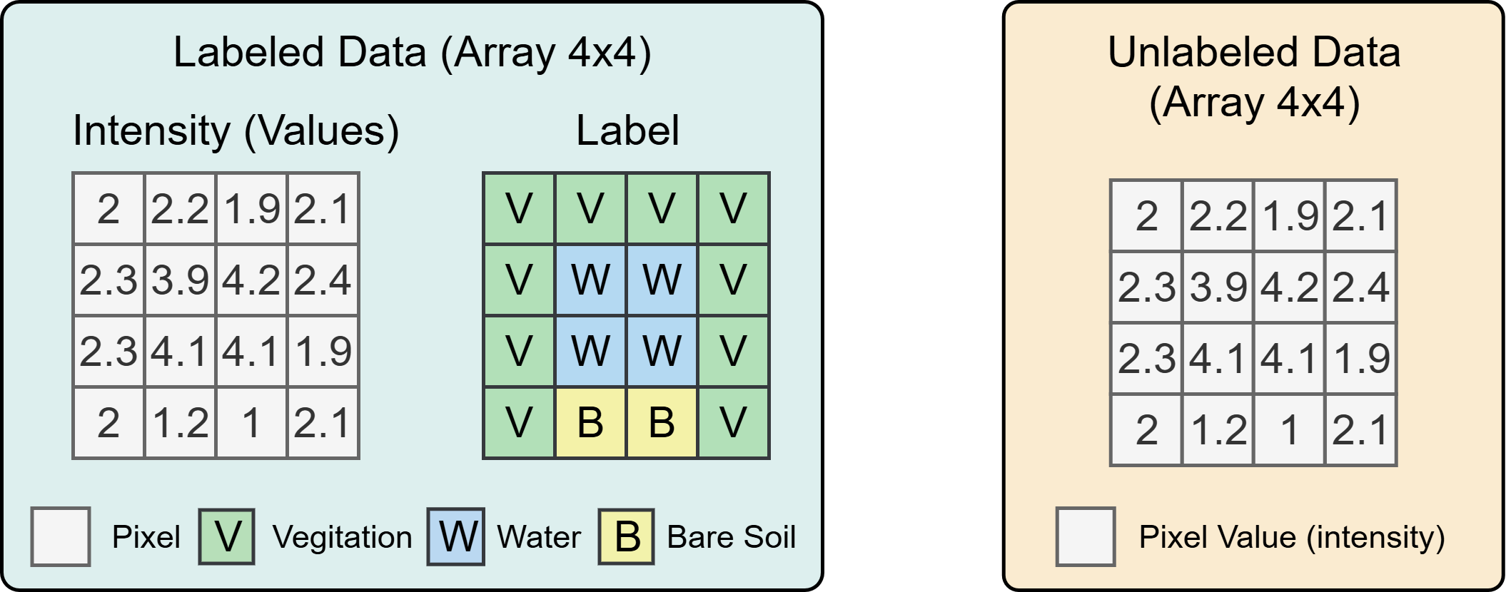
Figure 6:Labeled vs Unlabeled Data Structure for ML
Feature Engineering + ML
Together, feature engineering and machine learning form the analytical core of the hyperspectral workflow. Feature engineering improves the quality and relevance of the input variables, while machine learning uses those variables to generate meaningful outputs such as thematic maps, biophysical variable maps, and change-detection products.
Distinction Between Image Analysis and Image Interpretation
Two important concepts to understand are image analysis and image interpretation. Although these terms are related, they are not the same. Image analysis is concerned with extracting meaningful information from images using image processing methods. For example, in Module 1, we used a histogram to analyze band values, as shown in Figure 7. In general, image analysis tools are methods that work directly with image pixels and their intensity values.
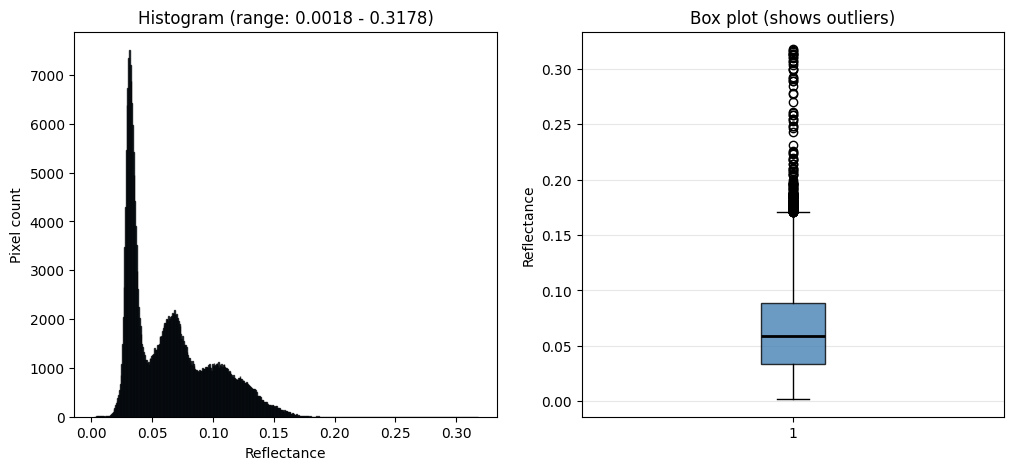
Figure 7:Histogram as an image analysis method
On the other hand, image interpretation is concerned with understanding the content of an image, such as identifying objects, recognizing patterns, and explaining what the scene represents. Tools used for image interpretation focus on assigning meaning to the image content. Examples include image classification and pattern recognition, which help identify objects and determine the overall meaning of the scene.
Remote Sensing Applications
Remote sensing applications can be organized according to the main analytical task rather than only by domain. The major task categories include classification, regression, segmentation, object detection, change detection, time-series forecasting and anomaly detection. Within each task category, applications span multiple domains such as agriculture, forestry, urban studies, hydrology, disaster management, climate monitoring, geology, and oceanography.