
Welcome to the first lesson of Module 3
In the previous lesson, we hand-picked a few “pure” looking pixels to study how light behaves. However, real-world remote sensing data is rarely perfect. It is often noisy and obstructed by clouds or shadows.
Before moving to extract insights and implement advanced analysis such as clustering or classification, we must build a preprocessing pipeline to refine our raw data into a “Analysis-Ready” state.
Data Acquisition
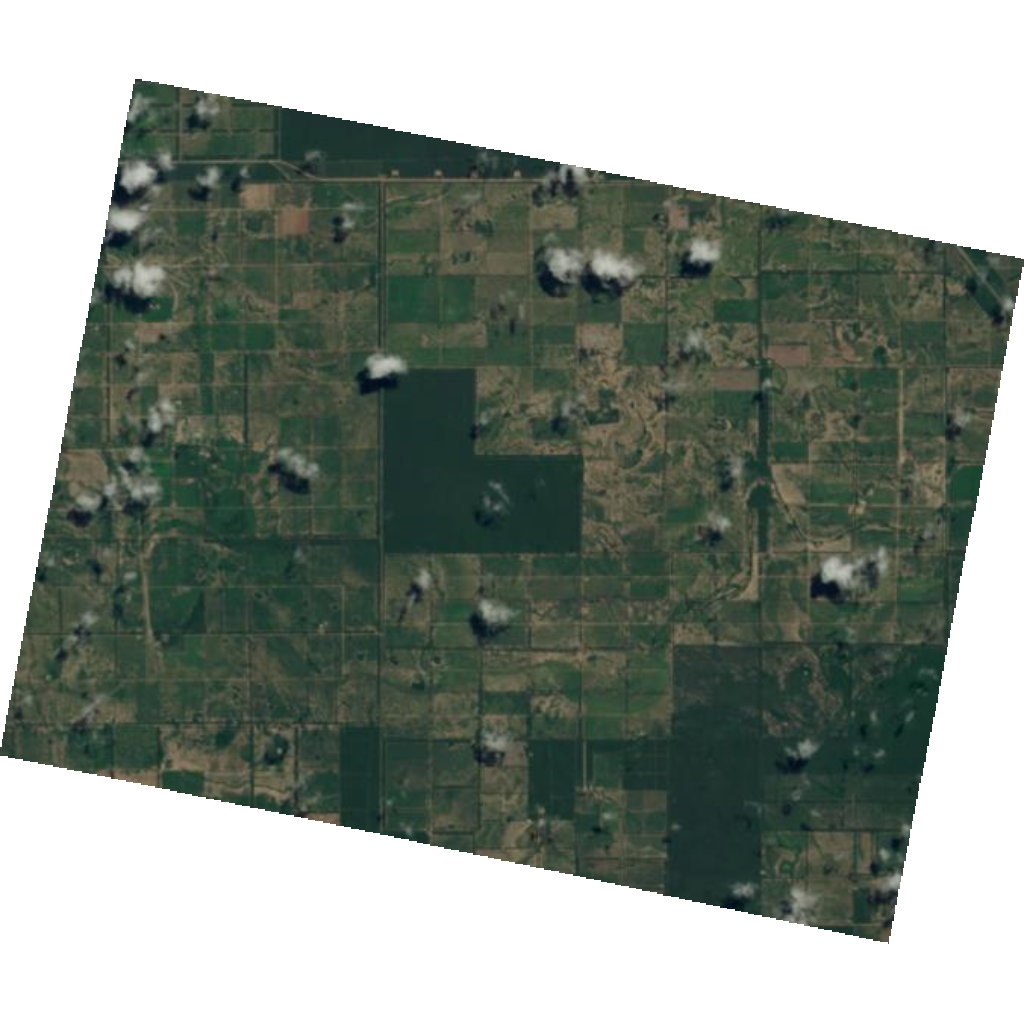
To practice building a cleaning pipeline, we need a dataset that is imperfect. We will download a specific Tanager-1 scene as shown below that contains clouds. We selected the Ortho surface reflectance scene.
🧰 Your Toolkit so far
You wrapped up Module 2 in Lesson 5, which added no new function — so the Toolkit below is exactly as it has stood since Module 2 · Lesson 4: print_structure, load_tanager_hdf5, nearest_band, and make_rgb. Keep it near the top and run it before anything else. By the end of this lesson you’ll upgrade load_hdf5 so it cleans the cube as it loads.
# Import essential libraries

import h5py
import numpy as np
import matplotlib.pyplot as plt
import matplotlib.patches as mpatches

# ---- setup -------------------------------------------------------------

def download_tanager_data(url, file_path):

    import os
    import urllib.request

    def _progress(count, block_size, total_size):
        mb_done = count * block_size / 1_000_000
        mb_total = total_size / 1_000_000
        print(f"\rDownloading... {mb_done:.1f} / {mb_total:.1f} MB", end="", flush=True)

    if not os.path.exists(file_path):
        urllib.request.urlretrieve(url, file_path, reporthook=_progress)
        print(f"\nDownload complete: {file_path}")
    else:
        print(f"File already exists, skipping download: {file_path}")
    return file_path

# ---- io ----------------------------------------------------------------

def print_structure(name, obj):

    level = name.count('/')
    indent = '    ' * level

    if isinstance(obj, h5py.Group):
        print(f"{indent}📂 {name}/")
    elif isinstance(obj, h5py.Dataset):
        print(f"{indent}📄 {name} | {obj.shape} | {obj.dtype}")

    if len(obj.attrs) > 0:
        for key, val in obj.attrs.items():
            val_str = str(val)
            if len(val_str) > 50:
                val_str = val_str[:50] + "..."
            print(f"{indent}    ↳ 🏷️ {key}: {val_str}")

def load_hdf5(file_path,
    data_path='HDFEOS/SWATHS/HYP/Data Fields/surface_reflectance',
    band=None
    ):

    with h5py.File(file_path, 'r') as f:
        dset = f[data_path]
        data = dset[:] if band is None else dset[band]
        attrs = dict(dset.attrs)
    return data, attrs

# ---- bands -------------------------------------------------------------

def nearest_band(wavelengths, target_nm):
    """Return the index of the band whose wavelength is closest to ``target_nm``.

    Parameters
    ----------
    wavelengths : ndarray
        Per-band center wavelengths (nm).
    target_nm : float
        Wavelength of interest (nm).

    Returns
    -------
    int
        Index of the nearest band.
    """
    return int(np.argmin(np.abs(np.asarray(wavelengths) - target_nm)))

# ---- visualization ----------------------------------------------------

def make_rgb(cube, wavelengths, r_nm=680, g_nm=560, b_nm=470,
             percentile_low=2, percentile_high=98):
    """Build a contrast-stretched true-colour RGB composite from a cube.

    Picks the bands nearest the three target wavelengths, stacks them, and
    applies a percentile stretch (computed with ``nanpercentile`` so NaN
    no-data is ignored).

    Parameters
    ----------
    cube : ndarray, shape (bands, rows, cols)
        Hyperspectral cube.
    wavelengths : ndarray
        Per-band center wavelengths (nm).
    r_nm, g_nm, b_nm : float
        Target wavelengths (nm) for the red, green, blue channels.
    percentile_low, percentile_high : float
        Percentiles for the contrast stretch.

    Returns
    -------
    ndarray, shape (rows, cols, 3)
        RGB image normalized to [0, 1].
    """
    r = nearest_band(wavelengths, r_nm)
    g = nearest_band(wavelengths, g_nm)
    b = nearest_band(wavelengths, b_nm)
    rgb = np.dstack((cube[r], cube[g], cube[b]))
    p_low, p_high = np.nanpercentile(rgb, (percentile_low, percentile_high))
    return np.clip((rgb - p_low) / (p_high - p_low), 0, 1)
# Download the Tanager-1 Ortho SR HDF5 file (a cloudy scene) using your Toolkit's
# download_tanager_data (defined in the Toolkit cell above).
url = "https://storage.googleapis.com/open-cogs/planet-stac/tanager1-release2-core-imagery/ortho_sr_hdf5/20250301_143913_32_4001_ortho_sr_hdf5.h5"
file_path = '20250301_143913_32_4001_ortho_sr_hdf5.h5'
download_tanager_data(url, file_path)File already exists, skipping download: 20250301_143913_32_4001_ortho_sr_hdf5.h5
'20250301_143913_32_4001_ortho_sr_hdf5.h5'Loading the Cube & Quality Masks
To build a cleaning pipeline, we must first extract the required datasets from the HDF5 file. The table below presents the datasets we will use in this lesson, including the hyperspectral cube and the relevant masking layers.
We have already identified the internal HDF5 paths for you. The following table shows where each dataset is stored within the file structure:
| Dataset Name | HDF5 Internal Path | Description |
|---|---|---|
| Surface Reflectance | HDFEOS/GRIDS/HYP/Data Fields/surface_reflectance | The primary hyperspectral image - surface reflectance. |
| Uncertainty | HDFEOS/GRIDS/HYP/Data Fields/surface_reflectance_uncertainty | The estimated uncertainty of the surface reflectance. |
| Beta Cloud Mask | HDFEOS/GRIDS/HYP/Data Fields/beta_cloud_mask | Binary mask (0/1) identifying the presence optically thick clouds. |
| Beta Cirrus Mask | HDFEOS/GRIDS/HYP/Data Fields/beta_cirrus_mask | Binary mask identifying the presence of thin, high-altitude clouds. |
| NoData Pixels | HDFEOS/GRIDS/HYP/Data Fields/nodata_pixels | Marks empty black corners (fill values) in the swath or pixels for which no data was recorded. |
Let’s now use these paths to load the data into Python.
# HDF5-EOS Internal Paths (Tanager-1 Standard)
path_sr  = "HDFEOS/GRIDS/HYP/Data Fields/surface_reflectance"

# Quality Masks
path_cloud  = "HDFEOS/GRIDS/HYP/Data Fields/beta_cloud_mask"
path_cirrus = "HDFEOS/GRIDS/HYP/Data Fields/beta_cirrus_mask"
path_nodata = "HDFEOS/GRIDS/HYP/Data Fields/nodata_pixels"

# 1. Load the cube + wavelengths with your Toolkit loader (simple version, raw cube)
sr_cube, attrs = load_hdf5(file_path, path_sr)

good_bands = attrs['good_wavelengths']
wavelengths = attrs['wavelengths']

# 2. Read the QA layers this lesson needs (the simple loader doesn't return them yet)
mask_cloud, attrs = load_hdf5(file_path, path_cloud)
mask_cirrus, attrs = load_hdf5(file_path, path_cirrus)
mask_nodata, attrs = load_hdf5(file_path, path_nodata)

# 3. Convert Fill Values to NaN immediately to prevent plotting errors
fill_value = attrs['_FillValue']
sr_cube[sr_cube == fill_value] = np.nan
Before Data Preprocessing
Before diving into preprocessing, it is essential to understand and familiarize yourself with your data.
This foundational step provides critical insights into data types and formats, which ultimately dictates how you will handle and manipulate the information throughout the pipeline.
# 1. Check Data Dimensions
# For Tanager-1, the shape is usually (Bands, Lines, Samples)
# though some APIs might transpose it.
n_bands, n_lines, n_samples = sr_cube.shape

print(f"--- Data Dimensions ---")
print(f"Number of Bands: {n_bands}")
print(f"Spatial Resolution (Lines x Samples): {n_lines} x {n_samples}")
print(f"Total Pixels: {n_lines * n_samples:,}")

# 2. Inspect Spectral Range
min_wl = np.min(wavelengths)
max_wl = np.max(wavelengths)
mean_spacing = np.mean(np.diff(wavelengths))

print(f"\n--- Spectral Information ---")
print(f"Wavelength Range: {min_wl:.2f} nm to {max_wl:.2f} nm")
print(f"Average Spectral Sampling: {mean_spacing:.2f} nm")

# 3. Identify 'Good' Bands
# Tanager uses a boolean or binary mask for bands unaffected by water vapor/noise
num_good = np.sum(good_bands)
print(f"Number of 'Good' Bands (Non-Atmospheric Absorption): {num_good} / {n_bands}")

# 4. Check Mask Statistics
# Understanding how much of your tile is actually usable (not cloud or nodata)
def get_mask_pct(mask):
    return (np.sum(mask > 0) / mask.size) * 100

print(f"\n--- Quality Assessment ---")
print(f"Cloud Cover: {get_mask_pct(mask_cloud):.2f}%")
print(f"Cirrus Cover: {get_mask_pct(mask_cirrus):.2f}%")
print(f"NoData Pixels: {get_mask_pct(mask_nodata):.2f}%")
--- Data Dimensions ---
Number of Bands: 426
Spatial Resolution (Lines x Samples): 680 x 805
Total Pixels: 547,400
--- Spectral Information ---
Wavelength Range: 376.44 nm to 2499.00 nm
Average Spectral Sampling: 4.99 nm
Number of 'Good' Bands (Non-Atmospheric Absorption): 368 / 426
--- Quality Assessment ---
Cloud Cover: 0.78%
Cirrus Cover: 0.00%
NoData Pixels: 30.40%
Data Preprocessing: Cleaning the Cube
With the data now loaded, we can begin cleaning the cube. In hyperspectral analysis, preprocessing is typically performed in a “Spectral-then-Spatial” sequence to preserve signal quality before modeling:
Spectral Pruning: Remove bands that appear noisy, as well as bands strongly affected by atmospheric absorption (for example, water-vapor regions).
Spatial Masking: Apply quality masks to exclude non-target pixels, such as clouds, dense shadows, and no-data areas, so downstream analysis uses only reliable, clear-ground reflectance.
Step 1: Remove “Bad” Bands (Spectral Pruning)
The Tanager-1 metadata includes a good_wavelengths attribute attached with the hyperspectral surface reflectance cube. This is a binary mask where:
1 (True): Identifies a usable band with high signal integrity.
0 (False): Identifies a “bad” band.
“Bad” bands are typically located in atmospheric water vapor absorption regions (around 1400 nm and 1900 nm). In these regions, the atmosphere absorbs almost all reflected solar energy, resulting in noise rather than signal. We must drop these bands to prevent them from skewing the analysis. This quality mask provided with each Tanager scene is a starting point. You may want to add or remove bands from the mask depending on your own analysis needs and the amount of water vapor noise present in a given image.
print(f"Original Cube Shape: {sr_cube.shape} (Bands, Height, Width)")

# 1. Identify valid indices
# We look for indices where the 'good_wavelengths' flag is set to 1.
valid_band_indices = np.where(good_bands == 1)[0]

# 2. Slice the Cube and Wavelengths
# We subset the cube along the first dimension (Bands)
# The spatial dimensions (Height, Width) remain untouched.
sr_cube_clean = sr_cube[valid_band_indices, :, :]
wavelengths_clean = wavelengths[valid_band_indices]

# 3. Verify the result
bands_removed = sr_cube.shape[0] - sr_cube_clean.shape[0]

print(f"Bands Removed: {bands_removed}")
print(f"New Cube Shape:  {sr_cube_clean.shape}")
print(f"Remaining Wavelengths: {len(wavelengths_clean)}")
Original Cube Shape: (426, 680, 805) (Bands, Height, Width)
Bands Removed: 58
New Cube Shape: (368, 680, 805)
Remaining Wavelengths: 368
Now, we are ready to Step 2: Spatial Masking, where you will tackle the other two dimensions.
Step 2: Generating and Applying a Composite “Bad Pixel” Mask
To streamline the workflow, we need to consolidate our masks or quality assurance (QA) layers. We have extracted three distinct masks from the Tanager-1 assets:
Clouds & Cirrus: Atmospheric obstructions that contaminate the spectral signal.
NoData (Ortho-Fill): These are geometric artifacts, not sensor errors. When the raw satellite swath (which is tilted relative to the map) is projected onto a north-up grid (orthorectification), the empty corners are filled with “NoData” values to maintain a rectangular file shape.
Managing these layers individually during analysis is inefficient. Instead, we will fuse them into a single Composite Mask. This binary filter acts as a “Gatekeeper” for our analysis:
0 (False): Valid Science Data (Pixels suitable for analysis).
1 (True): Invalid Data (Pixels to be excluded).
The Fusion Logic
By applying a logical OR operation, we ensure that if a pixel is flagged by any of the quality layers, it is marked as invalid in our final product:
# 1.Create the Composite Mask
# We use the Bitwise OR operator (|) which functions as the Union (∪)
combined_mask = (mask_cloud == 1) | (mask_cirrus == 1) | (mask_nodata == 1)

# 2. Apply the Mask
# We set invalid pixels to NaN (Not a Number).
# Note on Broadcasting:
# The mask is 2D (Lines, Samples). The cube is 3D (Bands, Lines, Samples).
# NumPy automatically applies this 2D mask to EVERY band in the cube.
sr_cube_masked = sr_cube_clean.copy()
sr_cube_masked[:, combined_mask] = np.nan

# 3. Calculate the percentage of true masked values
total_cloud_pixels = np.sum((mask_cloud == 1) | (mask_cirrus == 1))
total_pixels = sr_cube_masked.shape[1] * sr_cube_masked.shape[2]
true_total_pixels = total_pixels - np.sum(mask_nodata)
true_cloud_pct = (total_cloud_pixels / true_total_pixels) * 100
print(f"True Cloud Cover: {true_cloud_pct:.2f}%")
True Cloud Cover: 1.13%
Visualizing the Results
To gain a clear understanding of the Composite Mask and its impact on the data, we need to inspect the “before” and “after” states of the hyperspectral cube.
In this step, we generate a side-by-side comparison of the Composite Mask (the logic) and the Masked Cube (the final output). This visualization is a critical quality control (QC) step; it allows us to verify that clouds have been successfully isolated.
# Generate RGB composite and paint masked pixels yellow for visualization
rgb_masked = make_rgb(sr_cube_masked, wavelengths_clean, r_nm=680, g_nm=550, b_nm=470)
rgb_masked[combined_mask] = [1, 1, 0]  # Mark masked pixels as yellow

fig, axes = plt.subplots(1, 2, figsize=(16, 8), constrained_layout=True)

# Left: Show combined mask
im_mask = axes[0].imshow(combined_mask)
axes[0].set_title("Step 1: The Combined Mask\n(Yellow = Pixels to Remove)", fontsize=14)
axes[0].axis('off')

# Legend for mask plot
patches = [mpatches.Patch(color=im_mask.cmap(im_mask.norm(val)), label=lab) for val, lab in zip([0,1], ["Valid Data", "Masked Area"])]
axes[0].legend(handles=patches, loc='lower right', borderaxespad=0.5)

# Right: Show masked RGB composite
axes[1].imshow(rgb_masked)
axes[1].set_title("Step 2: Final RGB Composite\n(Yellow areas indicate removed data)", fontsize=14)
axes[1].axis('off')

plt.suptitle("Masking Validation: Visualizing Data Removal", fontsize=16, weight='bold')
plt.show()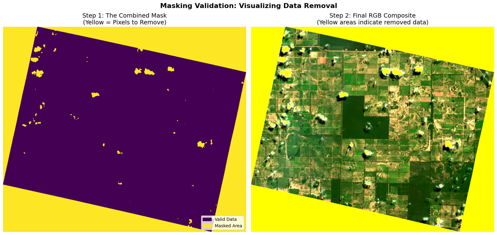
Let’s look closely at the plots above. The yellow regions in the Right Plot confirm that our pipeline successfully targeted the “NoData” edges and the large cloud formations. By removing these, we prevent them from skewing the minimum/maximum values of our dataset.
🧰 Toolkit Update: Teach Your Loader to Clean
You just cleaned the cube by hand. Two of those steps are universal — you’ll want them on every Tanager-1 load:
Drop the bad bands flagged by
good_wavelengths.Mask the
nodata_pixels(the orthorectification fill) toNaN.
Your next Toolkit upgrade folds both into load_hdf5. The loader gains a clean=True switch (plus a nodata_path) and now returns three things: data, attrs, no_data.
# =====================================================================
# 🧰 TOOLKIT — YOUR TURN  (implement before the next lesson)
# Fill in the body below; the reference solution appears at the top
# of the next coding lesson (Module 4 · Lesson 1, Part 2: Spectral Indices).
# =====================================================================
import h5py
import numpy as np

# ---- io ----------------------------------------------------------------

def load_hdf5(
    file_path,
    data_path='HDFEOS/GRIDS/HYP/Data Fields/surface_reflectance',
    nodata_path='HDFEOS/GRIDS/HYP/Data Fields/nodata_pixels',
    clean=True,
    band=None
    ):
    """Load a Tanager-1 hyperspectral cube (cleaning version).

    Upgraded in Module 3 · Lesson 1. With ``clean=True`` the two universal
    cleaning steps are applied: bad bands (``good_wavelengths == 0``) are
    dropped and ``nodata_pixels`` are set to NaN. Pass ``band=`` to read a
    single 2-D band straight from disk instead of the whole cube.

    Parameters
    ----------
    file_path : str
        Path to the Tanager-1 ``.h5`` file.
    data_path : str, optional
        Internal HDF5 path to the reflectance dataset (default: Ortho / GRIDS).
    nodata_path : str, optional
        Internal HDF5 path to the ``nodata_pixels`` mask.
    clean : bool, optional
        If True, drop bad bands and mask no-data pixels to NaN.
    band : int, optional
        If given, read only that band (a single 2-D slice) instead of the
        full cube — a quick, memory-light look at one wavelength.

    Returns
    -------
    data : ndarray
        Reflectance values: the full cube ``(bands, rows, cols)`` when
        ``band`` is None, otherwise a single ``(rows, cols)`` band. Bad
        bands are removed and no-data set to NaN when ``clean=True``.
    attrs : dict
        Dataset attributes, with ``'wavelengths'`` and ``'good_wavelengths'``
        trimmed to match ``data``.
    no_data : ndarray, shape (rows, cols), dtype=bool
        Boolean no-data mask.
    """
    # ------------------------------------------------------------------
    # HINTS — replace `pass` with your implementation
    # ------------------------------------------------------------------
    # 1) READ  (always)
    #    - Open the file with h5py and grab the dataset at data_path.
    #    - Read the whole cube when band is None, else a single slice
    #      dset[band]. Cast to float32 so the array can hold NaN.
    #    - Copy the attributes into a dict; pull out 'wavelengths' and
    #      'good_wavelengths' (a 0/1 flag per band).
    #    - Read the nodata_path mask as a boolean array.
    #
    # 2) CLEAN  (only when clean=True)
    #    Full cube (band is None) — exactly what you just did by hand:
    #      - keep only the good bands (boolean-index the band axis)
    #      - trim 'wavelengths' the same way
    #      - set the no-data pixels to NaN on every band
    #    Single band (band is given) — you hold just one 2-D slice:
    #      - if this band is NOT good, there is nothing to keep -> fill
    #        the whole slice with NaN
    #      - if it IS good, just NaN-out the no-data pixels
    #      - keep 'wavelengths'/'good_wavelengths' as 1-element arrays so
    #        the outputs still line up with the full-cube case
    #
    # 3) RETURN
    #    - Write the updated 'wavelengths' and 'good_wavelengths' back into
    #      attrs, then return  data, attrs, no_data

    # TODO: upgrade your simple loader into this cleaning version
    pass
Summary & Next Steps
In this lesson, we learned that hyperspectral data is never perfect out of the box. It contains empty edges, clouds, or unusable bands that can ruin a scientific analysis if left unchecked. By building a preprocessing pipeline, we successfully achieved our purpose for this tutorial.
Your Toolkit grew: load_hdf5 now cleans as it loads (returning data, attrs, no_data).
Now that our data is clean, we can extract insights and go with machine learning applications.
Next Up: In the next lesson, we will explore pathways for remote sensing applications. The “From Data to Insight” module introduces the roadmap from spectral indices to machine learning applications.
See you in the Lesson 2 of Module 3: From Data to Insight!