
Welcome to the first lesson in module 2.
In Lessons 2 and 3 of the previous module, we created a synthetic dataset and used it to learn the fundamental principles of HDF5.
In this lesson, we transition to working with real, operational Tanager-1 Science Data.
While the real data files are significantly larger and the hierarchy is more complex, the underlying mechanics remain identical. So, you will use the same workflows you have learned to work with real data.
Let’s begin!
Data Acquisition: Selecting a Scene
To analyze real data, we need to retrieve a sample from the Planet Tanager STAC Catalog.
💡 For this lesson, we’ve selected a specific scene and the Basic Surface Reflectance (
basic_sr_hdf5) asset so everyone follows the same example. Tanager-1 captures the full spectral fingerprint of the Earth across many domains (Agriculture, Water, Mineralogy, etc.). If you prefer a different theme or location, follow the Open Data STAC tutorial to pick your own scene, then either copy the asset URL into the download cell or download the file to your workspace. The workflow you learn here applies to any Tanager-1 data you choose.
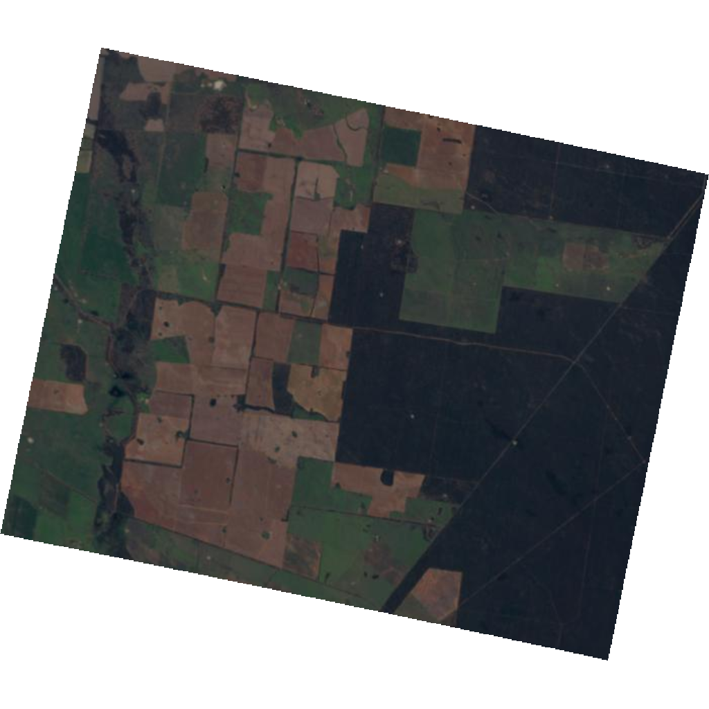
Pilliga, Narrabri Shire Council, New South Wales, 2388, Australia
# Essential imports for this lesson
import numpy as np              # For numerical operations and arrays
import h5py
import matplotlib.pyplot as plt # For creating plots and visualizations
import os                       # For operating system functionalities, e.g., file checks
# Download the Tanager-1 Basic SR HDF5 file
import urllib.request
url = "https://storage.googleapis.com/open-cogs/planet-stac/tanager1-release2-core-imagery/basic_sr_hdf5/20250510_005001_00_4001_basic_sr_hdf5.h5"
file_path = "20250510_005001_00_4001_basic_sr_hdf5.h5"
def _progress(count, block_size, total_size):
mb_done = count * block_size / 1_000_000
mb_total = total_size / 1_000_000
print(f"\rDownloading... {mb_done:.1f} / {mb_total:.1f} MB", end="", flush=True)
if not os.path.exists(file_path):
urllib.request.urlretrieve(url, file_path, reporthook=_progress)
print(f"\nDownload complete: {file_path}")
else:
print(f"File already exists, skipping download: {file_path}")
if not os.path.exists(file_path):
raise FileNotFoundError(
f"File '{file_path}' not found.\n"
"Please run the download cell above, or upload the file to your session."
)
print(f"File ready: {file_path}")File already exists, skipping download: 20250510_005001_00_4001_basic_sr_hdf5.h5
File ready: 20250510_005001_00_4001_basic_sr_hdf5.h5
Navigating Real Tanager-1 Hierarchies
As you remember from the previous lesson, if we tried to check f.keys() manually for every folder, it would take forever.
Instead, we will deploy an upgraded version of our Recursive Tree print_structure function.
What’s upgraded:
| Previous version | Upgraded version | |
|---|---|---|
| Shows | Path names only | Path names + Metadata (Attributes) for every object |
| Benefit | — | Inspect attributes on groups and datasets |
def print_structure(name, obj) -> None:
    """
    Enhanced Recursive Tree Viewer that prints structure AND metadata.
    """
    # 1. Calculate Indentation (Visual Depth)
    level = name.count('/')
    indent = '    ' * level

    # 2. Identify Type (Group or Dataset)
    if isinstance(obj, h5py.Group):
        icon = "📂"
        print(f"{indent}{icon} {name}/")
    elif isinstance(obj, h5py.Dataset):
        icon = "📄"
        # For datasets, we also print the shape/type
        print(f"{indent}{icon} {name} | {obj.shape} | {obj.dtype}")

    # 3. METADATA DUMP: Print all Attributes attached to this object
    # We use a distinct symbol (↳) to show these are "attributes"
    if len(obj.attrs) > 0:
        for key, val in obj.attrs.items():
            # Truncate very long attribute values to keep output readable
            val_str = str(val)
            if len(val_str) > 50:
                val_str = val_str[:50] + "..."

            print(f"{indent}    ↳ 🏷️ {key}: {val_str}")

# Note: We use the 'file_path' variable defined in the previous cell
print(f"--- 🕵️ Initiating Structural Audit of: {file_path} ---\n")

with h5py.File(file_path, 'r') as f:
    f.visititems(print_structure)
--- 🕵️ Initiating Structural Audit of: 20250510_005001_00_4001_basic_sr_hdf5.h5 ---
📂 HDFEOS/
📂 HDFEOS/ADDITIONAL/
📂 HDFEOS/ADDITIONAL/FILE_ATTRIBUTES/
📂 HDFEOS/SWATHS/
📂 HDFEOS/SWATHS/HYP/
↳ 🏷️ created_at: 2025-12-05T23:23:41.371559+00:00
↳ 🏷️ strip_id: 20250510_005001_00_4001_strip
📂 HDFEOS/SWATHS/HYP/Data Fields/
📄 HDFEOS/SWATHS/HYP/Data Fields/aerosol_optical_depth | (502, 607) | float32
↳ 🏷️ Unit: Unitless
↳ 🏷️ _FillValue: -9999.0
📄 HDFEOS/SWATHS/HYP/Data Fields/beta_cirrus_mask | (502, 607) | uint8
↳ 🏷️ _FillValue: 255
📄 HDFEOS/SWATHS/HYP/Data Fields/beta_cloud_mask | (502, 607) | uint8
↳ 🏷️ _FillValue: 255
📄 HDFEOS/SWATHS/HYP/Data Fields/column_water_vapour | (502, 607) | float32
↳ 🏷️ Unit: g/cm^2
↳ 🏷️ _FillValue: -9999.0
📄 HDFEOS/SWATHS/HYP/Data Fields/nodata_pixels | (502, 607) | uint8
↳ 🏷️ _FillValue: 255
📄 HDFEOS/SWATHS/HYP/Data Fields/sensor_azimuth | (502, 607) | float32
↳ 🏷️ Unit: Decimal Degrees
↳ 🏷️ _FillValue: -9999.0
📄 HDFEOS/SWATHS/HYP/Data Fields/sensor_to_ground_path_length | (502, 607) | float32
↳ 🏷️ Unit: Meters
↳ 🏷️ _FillValue: -9999.0
📄 HDFEOS/SWATHS/HYP/Data Fields/sensor_zenith | (502, 607) | float32
↳ 🏷️ Unit: Decimal Degrees
↳ 🏷️ _FillValue: -9999.0
📄 HDFEOS/SWATHS/HYP/Data Fields/sun_azimuth | (502, 607) | float32
↳ 🏷️ Unit: Decimal Degrees
↳ 🏷️ _FillValue: -9999.0
📄 HDFEOS/SWATHS/HYP/Data Fields/sun_zenith | (502, 607) | float32
↳ 🏷️ Unit: Decimal Degrees
↳ 🏷️ _FillValue: -9999.0
📄 HDFEOS/SWATHS/HYP/Data Fields/surface_reflectance | (426, 502, 607) | float32
↳ 🏷️ Unit: Unitless
↳ 🏷️ _FillValue: -9999.0
↳ 🏷️ fwhm: [5.39 5.42 5.45 5.48 5.52 5.55 5.58 5.6 5.63 5.66...
↳ 🏷️ fwhm_units: nm
↳ 🏷️ good_wavelengths: [1 1 1 1 1 1 1 1 1 1 1 1 1 1 1 1 1 1 1 1 1 1 1 1 1...
↳ 🏷️ wavelengths: [ 376.44 381.41 386.38 391.35 396.32 401.29 ...
↳ 🏷️ wavelengths_units: nm
📄 HDFEOS/SWATHS/HYP/Data Fields/surface_reflectance_uncertainty | (426, 502, 607) | float32
↳ 🏷️ Unit: Unitless
↳ 🏷️ _FillValue: -9999.0
📂 HDFEOS/SWATHS/HYP/Geolocation Fields/
↳ 🏷️ Planet_Ortho_Framing: {"cols": 775, "epsg_code": 32755, "geotransform": ...
📄 HDFEOS/SWATHS/HYP/Geolocation Fields/Latitude | (502, 607) | float64
↳ 🏷️ Unit: Decimal Degrees
↳ 🏷️ _FillValue: -9999.0
📄 HDFEOS/SWATHS/HYP/Geolocation Fields/Longitude | (502, 607) | float64
↳ 🏷️ Unit: Decimal Degrees
↳ 🏷️ _FillValue: -9999.0
📄 HDFEOS/SWATHS/HYP/Geolocation Fields/Time | (502,) | float64
↳ 🏷️ Unit: UTC
↳ 🏷️ _FillValue: -9999.0
📂 HDFEOS INFORMATION/
↳ 🏷️ HDFEOSVersion: b'HDFEOS_5.1.15'
📄 HDFEOS INFORMATION/StructMetadata.0 | () | |S32000
Interesting! Scroll through the output you just generated. You will see dozens of groups and datasets.
Do not get overwhelmed!
This is a standard HDF-EOS layout. Let’s break down exactly what we found.
The Roots
You will see two main groups within the root of HDF5 file: HDFEOS/ and HDFEOS INFORMATION/.
HDFEOS/: This is the most extensive group. It contains all the actual scientific datasets (📄).HDFEOS INFORMATION/: This largely contains structural metadata.
The Critical Paths
If you look closer at the map, you will find the two main groups that contain the data we most care about:
HDFEOS/SWATHS/HYP/Data Fields/: This holds the science data (Reflectance, Cloud Masks, etc.).HDFEOS/SWATHS/HYP/Geolocation Fields/: This holds the location data (Latitude, Longitude, Time).
The Attributes
The map also reveals the attributes (metadata). Remember, attributes are stored as Key-Value pairs.
Example: One of the attributes of the surface_reflectance dataset is named wavelengths (Key), and its value is a list of numbers representing the center wavelengths for each spectral band.
Understanding the Data Fields
Here is the breakdown of the HDFEOS/SWATHS/HYP/Data Fields/ group, organized into a single clear table.
Tanager Basic SR Data Fields
This helps you decide which datasets you actually need.
| Dataset name (HDF5 field) | Summary |
|---|---|
surface_reflectance | Category: Core Science Description: Bottom-of-Atmosphere (BOA) hyperspectral cube (Wavelengths x Rows x Columns) Primary Application: Deriving science products: Calculating vegetation indices, mapping minerals, and training classification models. |
surface_reflectance_uncertainty | Category: Quality Assurance Description: Per-pixel statistical uncertainty of the reflectance Primary Application: Evaluating data confidence: Understanding and incorporating the uncertainty of the estimated surface reflectance. |
beta_cloud_mask | Category: Masking Description: Binary mask indicating cloud presence (Beta product) Primary Application: Filtering usable data: Excluding cloud-obstructed pixels from spectral analysis. |
beta_cirrus_mask | Category: Masking Description: Binary mask for thin, semi-transparent clouds Primary Application: Filtering usable data: Identifying pixels where cirrus clouds might distort sensitive spectral bands. |
nodata_pixels | Category: Masking Description: Binary mask indicating missing or invalid sensor data Primary Application: Filtering usable data: Masking image edges or invalid measurements. |
aerosol_optical_depth | Category: Atmosphere Description: Measure of airborne particles (e.g., dust, smoke) Primary Application: Assessing atmospheric clarity: Understanding the relative thickness of aerosols estimated for each pixel. Note this is not currently a validated measurement. |
column_water_vapour | Category: Atmosphere Description: Total concentration of atmospheric water vapor present in the column Primary Application: Understanding atmospheric absorption: Seeing the amount of water vapor estimated to be in the atmosphere for each pixel. Note this is not currently a validated measurement. |
sun_zenith / sun_azimuth | Category: Geometry Description: Solar position (Zenith = degrees from nadir; Azimuth = degrees from N) Primary Application: Understanding illumination: Normalizing shadows, correcting terrain effects, and BRDF modeling. |
sensor_zenith / sensor_azimuth | Category: Geometry Description: Satellite viewing angle in degrees from nadir and orientation from north Primary Application: Correcting off-nadir effects: Adjusting for distortions when the satellite is not looking straight down. |
sensor_to_ground_path_length | Category: Geometry Description: The physical distance the light travels from the ground to the sensor Primary Application: Radiative transfer modeling: Used in advanced atmospheric correction algorithms. |
Data Extraction
Now that we know the paths, we can perform a targeted extraction. We will load two items:
The surface reflectance cube — the 3D array (bands × rows × columns)
The
wavelengthsattribute — metadata that tells us which band corresponds to which wavelength
# 1. Define Your Targets
# We store the path in a variable so it's easy to change later
DATA_PATH = 'HDFEOS/SWATHS/HYP/Data Fields/surface_reflectance'

with h5py.File(file_path, 'r') as f:

    # 2. Point to the Dataset
    dset = f[DATA_PATH]

    # 3. Extract Metadata (The Wavelengths)
    # We use .get() so the code is safe even if metadata is missing
    wavelengths = dset.attrs.get('wavelengths')

    # 4. Load the 3D Cube into RAM
    # The [:] syntax commands Python to read the ENTIRE dataset.
    # Note: For a 1GB file, this might take a few seconds.
    reflectance_cube = dset[:]

    # 5. Slice a band for visualization
    band_image = reflectance_cube[50,:,:]

# Print a summary of the loaded data and metadata
print(f"   - Cube Shape: {reflectance_cube.shape} (Bands, Height (rows), Width (columns))")
print(f"   - Wavelengths: Found {len(wavelengths)} bands")
- Cube Shape: (426, 502, 607) (Bands, Height (rows), Width (columns))
- Wavelengths: Found 426 bands
This is not the end — we are going to explore Tanager-1 data deeply and the other assets in the rest of this module.
Visualizing the Data
In the previous step, we extracted the full 3D cube and isolated a single 2D layer we named band_image (Band 50) for visualization.
Now, let’s visualize that specific slice.
# Retrieve Wavelength Info
# Let's find out what part of the spectrum Band 50 represents
band_idx = 50
band_wavelength = wavelengths[band_idx]

# Plot the image using gray colormap to represent reflectance intensity using default min and max values
plt.figure(figsize=(10, 8))
plt.imshow(band_image, cmap='gray')

plt.colorbar(label='Reflectance Intensity (0-1)')

# Dynamic Title: Shows the physical Wavelength, not just the index
plt.title(f"Tanager-1 Basic SR: Band {band_idx} ({band_wavelength:.1f} nm)\nShape: {band_image.shape}")
plt.xlabel("Sample (Column)")
plt.ylabel("Line (Row)")

plt.show()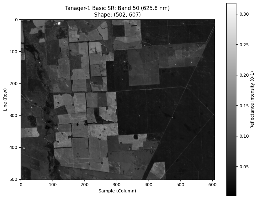
Bonus: Understanding Image Contrast
Did you notice the image may look faint, washed our, or lacking detail? Did you notice there is a single very bright pixel group at the top of the image, while the rest of the scene appears darker and flat?
What is happening? Because Tanager is highly sensitive, it captures a large dynamic range. A single scene can contain incredibly dark features right alongside very bright ones. Some pixels in the scene may have genuinely extreme reflectance values — bright surfaces like clouds, bare soil, or specular highlights can reflect much more light than surrounding vegetation or water. Even a small number of these outlier pixels is enough to pull the displayed maximum far above the typical scene values, compressing most of the landscape into a narrow, indistinguishable band of gray.
Why the image looks low-contrast by default
Most visualization tools map data values to grayscale like this:
the minimum value → black
the maximum value → white
If your array contains even a few unusually bright (or dark) outliers, the color mapping is forced to span that full range. As a result, the majority of pixels — the ones that actually represent the majority of the landscape — get squeezed into a narrow band of gray. That compression makes the image look flat and hides structure.
How plt.imshow() works?
When you call plt.imshow(band_image, cmap="gray"), Matplotlib has to convert your numeric values into screen brightness. It does this in two steps:
Normalize (scale) your data to a 0–1 range
Map 0 → black and 1 → white using the chosen colormap (here, grayscale)
By default, imshow() chooses the scaling limits from your array:
the minimum value → black (0)
the maximum value → white (1)
Figure 1 illustrates this mapping:
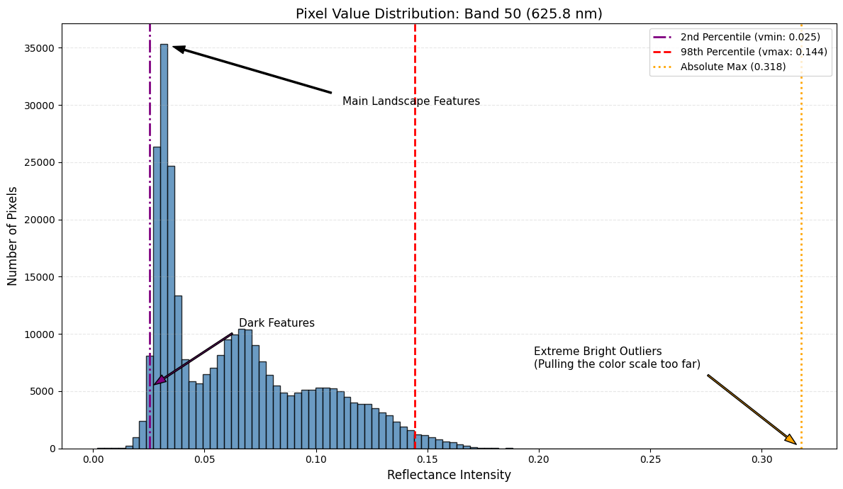
Figure 1:How imshow() maps data values to screen brightness by default: the array minimum becomes black and the array maximum becomes white. A single bright outlier forces the majority of pixels into a narrow, indistinguishable band of gray.
If your array contains even a few unusually bright (or dark) outliers, as was the case here, those extreme values become the max (or min).
How we fix it
To improve visibility, we usually don’t want to change the scientific values stored in band_image, those reflectance numbers are meaningful and should remain untouched for analysis.
Instead, we need to take control of our visual contrast. In practice, this is done by choosing better display limits plt.imshow():
vmin= the value we want to appear blackvmax= the value we want to appear white
Everything between vmin and vmax is stretched across the full grayscale range, and anything outside is clipped.
To choose good vmin and vmax, we first need to understand the distribution of reflectance values in band_image. So, we will plot a histogram and box-plot for the pixel values of the sliced band.
# Create a figure with two side-by-side plots: histogram and box plot
fig, (ax1, ax2) = plt.subplots(1, 2, figsize=(12, 5))

# Flatten the 2D band image into a 1D array so we can count how many pixels
# have each reflectance value (required for histogram)
flatten_image = band_image.flatten()

# each bar shows how many pixels fall within that interval
ax1.hist(flatten_image, bins=500, color='steelblue', alpha=0.8)

ax1.set_xlabel('Reflectance')
ax1.set_ylabel('Pixel count')
ax1.set_title(f'Histogram (range: {flatten_image.min():.4f} - {flatten_image.max():.4f})')

# Right: Box plot - clearly shows median, quartiles, and outliers
ax2.boxplot(flatten_image, vert=True, patch_artist=True,
            boxprops=dict(facecolor='steelblue', alpha=0.8),
            medianprops=dict(color='black', linewidth=2))
ax2.set_ylabel('Reflectance')
ax2.set_title('Box plot (shows outliers)')
ax2.grid(axis='y', alpha=0.3)
plt.tight_layout()
plt.show()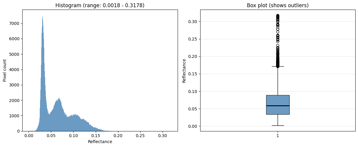
Interpreting the histogram
Interesting! The histogram reveals several important patterns, especially the distribution of values spanning roughly 0.0018 → 0.3178. From the histogram, we can see that:
Most pixels are concentrated in a relatively small range (the tall cluster on the left and the main body of the distribution).
The distribution is not uniform; it is multi-modal (it has several bumps/peaks). This confirms that the image likely contains multiple land-cover types with different reflectance characteristics.
There is a long right tail extending toward higher reflectance values. These pixels are relatively rare, but they push the maximum value upward.
While the histogram gives us a strong sense of the overall distribution, the box plot confirms the outlier behavior: the upper whisker reaches into the brighter part of the scene, and the many points above it are outliers. These outliers extend up toward the maximum (~0.32), meaning there are some very bright pixels compared to the rest of the image.
Why this matters for contrast
Now we can see why the default image looked faint, as we mentioned imshow() by default maps min → black and max → white. So, in our case the maximum is pulled upward by a small number of very bright outliers. That forces the majority of pixels (the landscape signal) to occupy only a small fraction of the grayscale, making the image look flat and low-contrast.
What we do next
Instead of using the absolute minimum and maximum, we will choose vmin and vmax from the main bulk of the distribution, typically using percentiles (e.g., the 2nd and 98th, or the 1st and 99th). This prevents rare outliers from dominating the display scaling and allows most landscape pixels to spread across the full grayscale range.
Next, we’ll compute percentiles and use them for plt.imshow(..., vmin=..., vmax=...), then compare the old plot with the new one.
# Calculate percentiles
p_02, p_98 = np.percentile(band_image, (2,98))

# Plot the maps
fig, (normal_plot, stretched_plot) = plt.subplots(1, 2, figsize=(14, 5))

normal_plot.imshow(band_image, cmap='gray')
normal_plot.set_title(f"Default Map")
normal_plot.axis("off")

stretched_plot.imshow(band_image, cmap='gray', vmin=p_02, vmax=p_98)
stretched_plot.set_title(f"Stretched (2–98%)")
stretched_plot.axis("off")

fig.tight_layout()
plt.show()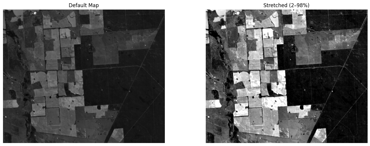
Notice the difference: the 2–98% stretch dramatically improves contrast. Field boundaries, texture, and subtle land-cover transitions that were hidden or difficult to see in the default view become clearly visible.
Beyond contrast: using vmin/vmax to explore the data
So far, we used vmin and vmax to improve the visual contrast of the image. But this same technique is useful for something even more powerful: data exploration.
By deliberately choosing a narrow value range (a “window”), we can make the map behave like a highlight tool:
Pixels inside the chosen range become visible and detailed.
Pixels outside the range get clipped to black or white and become less informative.
This helps us isolate and inspect specific reflectance ranges that may correspond to different surface types.
In other words, this isn’t only about “making the image prettier”, it’s a way to connect the histogram to the geography.
Why this works especially well here (multi-modal histogram)
Our histogram is multi-modal, meaning it has several peaks. In remote sensing, this often happens because the scene contains multiple land-cover types, each with its own typical reflectance range (for example: water, vegetation, bare soil, built-up areas, clouds, etc.).
Each “bump” in the histogram is often a mixture of one or more surface classes. By selecting a small window around a peak—and plotting the map using that same window, we can start answering questions like:
Where are the pixels that belong to this peak located?
What land features do they represent?
Does this peak correspond to fields, roads, water, or something else?
Let’s explore the strongest peak
Looking at the histogram, the tallest spike contains a huge number of pixels. That makes it a perfect starting point: it likely represents the dominant surface type in the scene.
In this next step, we’ll “zoom in” on that peak by choosing a tight vmin/vmax window (like 0.019 → 0.040) and then plotting:
The spatial map using that window
The histogram showing exactly which part of the distribution we are viewing
# Set a vmin/vmax value based on the portion of the histogram we want to focus on.
vmin = 0.019
vmax = 0.04

# Plot: Map + Value Distribution (histogram)
# The histogram shows what values we're plotting—helps verify data range, spot outliers, and interpret the map.
fig, (ax_map, ax_hist) = plt.subplots(1, 2, figsize=(14, 5))

# Left: The map
im = ax_map.imshow(band_image, cmap='gray', vmin=vmin, vmax=vmax)
plt.colorbar(im, ax=ax_map, label='Reflectance Intensity (0-1)')
ax_map.set_title(f"Band 50 ({band_wavelength:.1f} nm)\nShape: {band_image.shape}")
ax_map.set_xlabel("Sample (Column)")
ax_map.set_ylabel("Line (Row)")

# Right: Distribution of pixel values
ax_hist.hist(band_image.flatten(), bins=500, color='steelblue', alpha=0.8)
ax_hist.axvline(vmin, color='orange', linestyle='--', label=f'vmin ({vmin:.3f})')
ax_hist.axvline(vmax, color='red', linestyle='--', label=f'vmax ({vmax:.3f})')
ax_hist.set_xlabel('Reflectance')
ax_hist.set_ylabel('Pixel count')
ax_hist.set_title('Value distribution')
ax_hist.legend()

plt.suptitle('Tanager-1 Basic SR: Band 50', fontsize=12, y=1.02)
plt.tight_layout()
plt.show()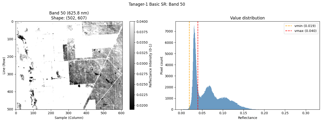
Can you see what happened? By focusing on this narrow reflectance window, we’ve revealed fine spatial detail that was previously buried in very dark gray tones. Features that looked nearly uniform in the default view now separate into distinct textures and boundaries. That’s the real power of histogram-guided visualization: it helps you connect value ranges to real land patterns.
I encourage you to experiment:
Move the window to the next bump in the histogram
Try a window over the right tail (brighter surfaces)
Try a window over the dark tail (very low-reflectance features)
Each time you shift the window, ask yourself: Which parts of the scene become clearer now—and what might they represent? This is how you translate histogram peaks into meaningful land features.
🧰 Starting Your Toolkit
You just used two pieces of code that you will reach for in every remaining lesson:
print_structure— audit any Tanager-1 HDF5 file’s hierarchy and attributes.The loading recipe — open the file, point at a dataset, read its values, and read its attributes (here, the
wavelengths).
This is the course’s build-your-own-toolkit assignment. Instead of re-typing these every time, you will package them into reusable functions kept in a single Toolkit cell that grows lesson by lesson, by the end of the course it is your own hyperspectral analysis library.
Below is the skeleton of your first two tools: print_structure and a general loader, load_hdf5. The signatures and docstrings are given, your job is to fill in the bodies using the code you wrote above. Notice the loader is written to generalize that recipe: rather than hard-coding the surface_reflectance cube and the single wavelengths attribute, it loads any dataset at data_path and hands back its data plus all of its properties (attributes) as a dict, so the very same function will later load masks, geometry layers, and Ortho cubes without a rewrite. An optional band= argument lets it lazily read a single 2-D band straight from disk when you don’t need the whole cube.
Your Toolkit also starts with one function we wrote for you: download_tanager_data, the packaged version of the download cell you ran above. You don’t implement this one, just call it at the top of every lesson that needs data. It travels with your Toolkit from the next lesson on.
Provided for you: download_tanager_data
You don’t implement this one, it’s the packaged version of the download cell you ran at the top of this lesson. It fetches a scene’s .h5 file (and skips the download when the file is already on disk). Keep it at the top of your Toolkit and call it whenever a lesson needs data.
def download_tanager_data(url, file_path):
    """Download a Tanager-1 data file to disk if it isn't already there.

    Provided for you — you don't need to implement this one. It streams the file
    from ``url`` to ``file_path`` with a simple MB progress readout and skips the
    download when the file already exists, so re-running a lesson stays cheap.
    Returns ``file_path`` so you can hand it straight to ``load_tanager_hdf5``.

    Parameters
    ----------
    url : str
        Public URL of the ``.h5`` file.
    file_path : str
        Local filename to save to (also checked before downloading).

    Returns
    -------
    str
        The local ``file_path``, ready to load.
    """
    import os
    import urllib.request

    def _progress(count, block_size, total_size):
        mb_done = count * block_size / 1_000_000
        mb_total = total_size / 1_000_000
        print(f"\rDownloading... {mb_done:.1f} / {mb_total:.1f} MB", end="", flush=True)

    if not os.path.exists(file_path):
        urllib.request.urlretrieve(url, file_path, reporthook=_progress)
        print(f"\nDownload complete: {file_path}")
    else:
        print(f"File already exists, skipping download: {file_path}")
    return file_path
# =====================================================================
# 🧰 TOOLKIT — YOUR TURN (implement before the next lesson)
# Fill in the bodies below; the reference solution appears at the top
# of the next coding lesson (Module 2 · Lesson 3: Basic vs Ortho).
# =====================================================================
# Import necessary libraries
import h5py
import numpy as np
# ---- io ----------------------------------------------------------------
def print_structure(name, obj):
"""
Print one HDF5 object (group or dataset) plus its attributes.
Designed as a callback for ``h5py.File.visititems`` to render the full
hierarchy of a Tanager-1 file as an indented tree.
Parameters
----------
name : str
Full HDF5 path of the object (provided by ``visititems``).
obj : h5py.Group or h5py.Dataset
The object itself (provided by ``visititems``).
"""
# TODO: indent by depth (count '/'); print groups as "📂 name/" and
# datasets as "📄 name | shape | dtype"; then dump each object's
# attributes on indented "↳ 🏷️ key: value" lines.
pass
def load_hdf5(
file_path,
data_path='HDFEOS/SWATHS/HYP/Data Fields/surface_reflectance',
band=None):
"""Load a dataset (or one band) from a Tanager-1 HDF5 file, with its properties.
Works for ANY dataset in the file — reflectance cubes, masks, geometry layers —
because it never assumes what the values mean. Pass ``band`` to lazily read a
single 2-D band straight from disk (cheap on RAM); leave it ``None`` for the
full array.
Parameters
----------
file_path : str
Path to the Tanager-1 ``.h5`` file.
data_path : str, optional
Internal HDF5 path to the dataset (Basic ``…/SWATHS/…`` by default; switch
to ``…/GRIDS/…`` for Ortho, or to any mask / geometry layer).
band : int, optional
If given, read only that band index (lazy slice); if ``None``, read all.
Returns
-------
data : ndarray
The full array, or a single 2-D band if ``band`` is given.
attrs : dict
All attributes (properties) of the dataset — e.g. ``'wavelengths'``,
``'units'``, ``'good_wavelengths'``.
"""
# TODO: open file_path with h5py; select the dataset at data_path; read the whole
# array, or just dset[band] when band is not None, into `data`; copy the
# dataset's attributes into a dict `attrs`; return (data, attrs).
passSummary & Next Steps
Congratulations. You have successfully navigated the transition from synthetic training data to Operational Satellite Imagery.
In this lesson, you achieved four critical milestones:
Acquisition: You retrieved a massive Tanager-1 dataset from Planet’s Open STAC catalog.
Audit: You used recursive mapping to penetrate the complex HDF-EOS hierarchy.
Extraction: You identified the key dataset in the file—the Reflectance Cube and its spectral wavelengths.
Visualization: You converted raw 3D arrays into a visible map of the Earth’s surface.
…and you started your Toolkit with print_structure and load_tanager_hdf5.
But we ignored something important.
When you looked at the STAC Catalog, you saw a confusing list of other files: ortho_reflectance, basic_radiance, geolocation_array.
Should you use Basic or Ortho?
Do you need Radiance or Reflectance?
Next Up: In the next lesson, we will decode the Tanager-1 asset ecosystem. We will learn exactly which file to pick for your specific science goal and how to use the Visual and UDM assets to quality-check your data before you process it.
See you in Lesson 2 of Module 2: The Tanager-1 Asset Ecosystem!