
Welcome to the third lesson in module 2.
In the previous lesson, you learned how to choose between Basic and Ortho assets. Here, we put that knowledge into practice: we’ll load both geometries for the same scene and compare them side-by-side. By the end, you’ll see exactly how the raw sensor view (Basic) differs from the map-projected view (Ortho).
Download the Assets
We’ll use a scene over Ringkøbing-Skjern, Denmark, with varied land cover, water, bare soil, and vegetation, so the geometric differences are easy to spot. Download both basic_sr_hdf5 and ortho_sr_hdf5 for the scene shown below.
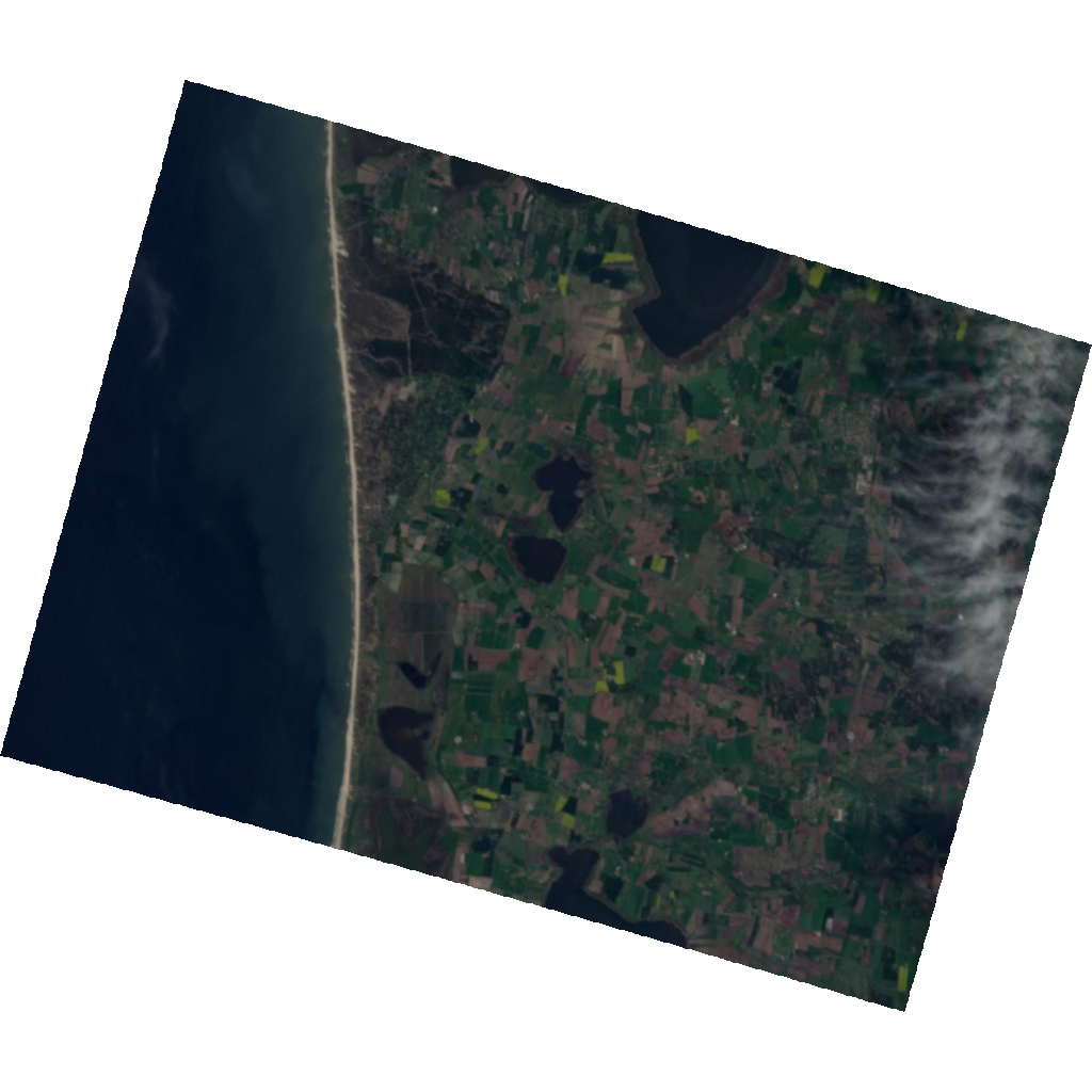
All data products from Tanager-1 for 20250510_112042_16_4001 near Ringkøbing-Skjern Municipality, Central Denmark Region, Denmark.
🧰 Your Toolkit so far
You started your Toolkit in Module 2 · Lesson 1 with print_structure and load_tanager_hdf5. The cell below is the reference solution, compare it with the versions you implemented as last lesson’s challenge. Keep this cell near the top of every notebook from now on and run it before anything else; you’ll keep adding to it as the course goes on.
# ==================
# 🧰 YOUR TOOLKIT
# ==================

# Essential imports for this lesson
import h5py
import numpy as np
import matplotlib.pyplot as plt


# ---- setup -------------------------------------------------------------

def download_tanager_data(url, file_path):
    import os
    import urllib.request

    def _progress(count, block_size, total_size):
        mb_done = count * block_size / 1_000_000
        mb_total = total_size / 1_000_000
        print(f"\rDownloading... {mb_done:.1f} / {mb_total:.1f} MB", end="", flush=True)

    if not os.path.exists(file_path):
        urllib.request.urlretrieve(url, file_path, reporthook=_progress)
        print(f"\nDownload complete: {file_path}")
    else:
        print(f"File already exists, skipping download: {file_path}")
    return file_path

# ---- io ----------------------------------------------------------------

def print_structure(name, obj):
    """Print one HDF5 object (group or dataset) plus its attributes.

    Designed as a callback for ``h5py.File.visititems`` to render the full
    hierarchy of a Tanager-1 file as an indented tree.

    Parameters
    ----------
    name : str
        Full HDF5 path of the object (provided by ``visititems``).
    obj : h5py.Group or h5py.Dataset
        The object itself (provided by ``visititems``).
    """
    level = name.count('/')
    indent = '    ' * level

    if isinstance(obj, h5py.Group):
        print(f"{indent}📂 {name}/")
    elif isinstance(obj, h5py.Dataset):
        print(f"{indent}📄 {name} | {obj.shape} | {obj.dtype}")

    if len(obj.attrs) > 0:
        for key, val in obj.attrs.items():
            val_str = str(val)
            if len(val_str) > 50:
                val_str = val_str[:50] + "..."
            print(f"{indent}    ↳ 🏷️ {key}: {val_str}")

def load_hdf5(file_path,
                      data_path='HDFEOS/SWATHS/HYP/Data Fields/surface_reflectance',
                      band=None):
    """Load a dataset (or one band) from a Tanager-1 HDF5 file, with its properties.

    Works for ANY dataset in the file — reflectance cubes, masks, geometry layers —
    because it never assumes what the values mean. Pass ``band`` to lazily read a
    single 2-D band straight from disk (cheap on RAM); leave it ``None`` for the
    full array.

    Parameters
    ----------
    file_path : str
        Path to the Tanager-1 ``.h5`` file.
    data_path : str, optional
        Internal HDF5 path to the dataset (Basic ``…/SWATHS/…`` by default; switch
        to ``…/GRIDS/…`` for Ortho, or to any mask / geometry layer).
    band : int, optional
        If given, read only that band index (lazy slice); if ``None``, read all.

    Returns
    -------
    data : ndarray
        The full array, or a single 2-D band if ``band`` is given.
    attrs : dict
        All attributes (properties) of the dataset — e.g. ``'wavelengths'``,
        ``'units'``, ``'good_wavelengths'``.
    """
    with h5py.File(file_path, 'r') as f:
        dset = f[data_path]
        data = dset[:] if band is None else dset[band]
        attrs = dict(dset.attrs)
return data, attrs# Download the Basic and Ortho SR assets for this scene using your Toolkit's
# download_tanager_data (defined in the Toolkit cell above).
basic_sr_url = "https://storage.googleapis.com/open-cogs/planet-stac/tanager1-release2-core-imagery/basic_sr_hdf5/20250510_112042_16_4001_basic_sr_hdf5.h5"
ortho_sr_url = "https://storage.googleapis.com/open-cogs/planet-stac/tanager1-release2-core-imagery/ortho_sr_hdf5/20250510_112042_16_4001_ortho_sr_hdf5.h5"
# These filenames are reused throughout the lesson:
# Note: You can change the file name to any name you want.
basic_sr_path = "20250510_112042_16_4001_basic_sr_hdf5.h5"
ortho_sr_path = "20250510_112042_16_4001_ortho_sr_hdf5.h5"
download_tanager_data(basic_sr_url, basic_sr_path)
download_tanager_data(ortho_sr_url, ortho_sr_path)
print("✅ Assets ready")File already exists, skipping download: 20250510_112042_16_4001_basic_sr_hdf5.h5
File already exists, skipping download: 20250510_112042_16_4001_ortho_sr_hdf5.h5
✅ Assets ready
Accessing the Hyperspectral Cubes
To read the hyperspectral data from an HDF5 file, we need the exact path to the dataset inside the file, just as we did in the first lesson of this module. However, we cannot reuse the data path from that lesson here.
Why? The internal structure of Tanager-1 HDF5 files differs depending on the geometry:
Basic files organize data under a SWATH group, which represents the raw satellite strip (sensor geometry).
Ortho files organize data under a GRID group, which represents the map-projected view.
Because Basic and Ortho use different root structures, the paths to the reflectance cube are not the same. Before we load the cubes, let’s use a lightweight Tree Viewer print_structure to locate the exact path for each file.
What to Look For
Scroll through the tree output for each file. You’ll see a key structural difference at the top level:
Basic file: The data lives under
HDFEOS/SWATHS/...— this confirms you’re looking at raw swath (sensor) geometry.Ortho file: The data lives under
HDFEOS/GRIDS/...— this confirms you’re looking at projected grid (map) geometry.
Inside each structure, locate the surface_reflectance dataset. Copy the full path to that dataset for both the Basic and Ortho files, we’ll use these paths in the next step to load the hyperspectral cubes.
# Basic Surface Reflectance
with h5py.File(basic_sr_path, 'r') as f:
    f.visititems(print_structure)
📂 HDFEOS/
📂 HDFEOS/ADDITIONAL/
📂 HDFEOS/ADDITIONAL/FILE_ATTRIBUTES/
📂 HDFEOS/SWATHS/
📂 HDFEOS/SWATHS/HYP/
↳ 🏷️ created_at: 2025-12-05T23:23:55.300666+00:00
↳ 🏷️ strip_id: 20250510_112038_00_4001_strip
📂 HDFEOS/SWATHS/HYP/Data Fields/
📄 HDFEOS/SWATHS/HYP/Data Fields/aerosol_optical_depth | (501, 607) | float32
↳ 🏷️ Unit: Unitless
↳ 🏷️ _FillValue: -9999.0
📄 HDFEOS/SWATHS/HYP/Data Fields/beta_cirrus_mask | (501, 607) | uint8
↳ 🏷️ _FillValue: 255
📄 HDFEOS/SWATHS/HYP/Data Fields/beta_cloud_mask | (501, 607) | uint8
↳ 🏷️ _FillValue: 255
📄 HDFEOS/SWATHS/HYP/Data Fields/column_water_vapour | (501, 607) | float32
↳ 🏷️ Unit: g/cm^2
↳ 🏷️ _FillValue: -9999.0
📄 HDFEOS/SWATHS/HYP/Data Fields/nodata_pixels | (501, 607) | uint8
↳ 🏷️ _FillValue: 255
📄 HDFEOS/SWATHS/HYP/Data Fields/sensor_azimuth | (501, 607) | float32
↳ 🏷️ Unit: Decimal Degrees
↳ 🏷️ _FillValue: -9999.0
📄 HDFEOS/SWATHS/HYP/Data Fields/sensor_to_ground_path_length | (501, 607) | float32
↳ 🏷️ Unit: Meters
↳ 🏷️ _FillValue: -9999.0
📄 HDFEOS/SWATHS/HYP/Data Fields/sensor_zenith | (501, 607) | float32
↳ 🏷️ Unit: Decimal Degrees
↳ 🏷️ _FillValue: -9999.0
📄 HDFEOS/SWATHS/HYP/Data Fields/sun_azimuth | (501, 607) | float32
↳ 🏷️ Unit: Decimal Degrees
↳ 🏷️ _FillValue: -9999.0
📄 HDFEOS/SWATHS/HYP/Data Fields/sun_zenith | (501, 607) | float32
↳ 🏷️ Unit: Decimal Degrees
↳ 🏷️ _FillValue: -9999.0
📄 HDFEOS/SWATHS/HYP/Data Fields/surface_reflectance | (426, 501, 607) | float32
↳ 🏷️ Unit: Unitless
↳ 🏷️ _FillValue: -9999.0
↳ 🏷️ fwhm: [5.39 5.42 5.45 5.48 5.52 5.55 5.58 5.6 5.63 5.66...
↳ 🏷️ fwhm_units: nm
↳ 🏷️ good_wavelengths: [1 1 1 1 1 1 1 1 1 1 1 1 1 1 1 1 1 1 1 1 1 1 1 1 1...
↳ 🏷️ wavelengths: [ 376.44 381.41 386.38 391.35 396.32 401.29 ...
↳ 🏷️ wavelengths_units: nm
📄 HDFEOS/SWATHS/HYP/Data Fields/surface_reflectance_uncertainty | (426, 501, 607) | float32
↳ 🏷️ Unit: Unitless
↳ 🏷️ _FillValue: -9999.0
📂 HDFEOS/SWATHS/HYP/Geolocation Fields/
↳ 🏷️ Planet_Ortho_Framing: {"cols": 847, "epsg_code": 32632, "geotransform": ...
📄 HDFEOS/SWATHS/HYP/Geolocation Fields/Latitude | (501, 607) | float64
↳ 🏷️ Unit: Decimal Degrees
↳ 🏷️ _FillValue: -9999.0
📄 HDFEOS/SWATHS/HYP/Geolocation Fields/Longitude | (501, 607) | float64
↳ 🏷️ Unit: Decimal Degrees
↳ 🏷️ _FillValue: -9999.0
📄 HDFEOS/SWATHS/HYP/Geolocation Fields/Time | (501,) | float64
↳ 🏷️ Unit: UTC
↳ 🏷️ _FillValue: -9999.0
📂 HDFEOS INFORMATION/
↳ 🏷️ HDFEOSVersion: b'HDFEOS_5.1.15'
📄 HDFEOS INFORMATION/StructMetadata.0 | () | |S32000
# Ortho Surface Reflectance
with h5py.File(ortho_sr_path, 'r') as f:
    f.visititems(print_structure)
📂 HDFEOS/
📂 HDFEOS/ADDITIONAL/
📂 HDFEOS/ADDITIONAL/FILE_ATTRIBUTES/
📂 HDFEOS/GRIDS/
📂 HDFEOS/GRIDS/HYP/
↳ 🏷️ created_at: 2025-12-05T23:23:28.275751+00:00
↳ 🏷️ epsg_code: 32632
↳ 🏷️ strip_id: 20250510_112038_00_4001_strip
📂 HDFEOS/GRIDS/HYP/Data Fields/
📄 HDFEOS/GRIDS/HYP/Data Fields/aerosol_optical_depth | (724, 847) | float32
↳ 🏷️ Unit: Unitless
↳ 🏷️ _FillValue: -9999.0
📄 HDFEOS/GRIDS/HYP/Data Fields/beta_cirrus_mask | (724, 847) | uint8
↳ 🏷️ _FillValue: 255
📄 HDFEOS/GRIDS/HYP/Data Fields/beta_cloud_mask | (724, 847) | uint8
↳ 🏷️ _FillValue: 255
📄 HDFEOS/GRIDS/HYP/Data Fields/column_water_vapour | (724, 847) | float32
↳ 🏷️ Unit: g/cm^2
↳ 🏷️ _FillValue: -9999.0
📄 HDFEOS/GRIDS/HYP/Data Fields/nodata_pixels | (724, 847) | uint8
↳ 🏷️ _FillValue: 255
📄 HDFEOS/GRIDS/HYP/Data Fields/sensor_azimuth | (724, 847) | float32
↳ 🏷️ Unit: Decimal Degrees
↳ 🏷️ _FillValue: -9999.0
📄 HDFEOS/GRIDS/HYP/Data Fields/sensor_to_ground_path_length | (724, 847) | float32
↳ 🏷️ Unit: Meters
↳ 🏷️ _FillValue: -9999.0
📄 HDFEOS/GRIDS/HYP/Data Fields/sensor_zenith | (724, 847) | float32
↳ 🏷️ Unit: Decimal Degrees
↳ 🏷️ _FillValue: -9999.0
📄 HDFEOS/GRIDS/HYP/Data Fields/sun_azimuth | (724, 847) | float32
↳ 🏷️ Unit: Decimal Degrees
↳ 🏷️ _FillValue: -9999.0
📄 HDFEOS/GRIDS/HYP/Data Fields/sun_zenith | (724, 847) | float32
↳ 🏷️ Unit: Decimal Degrees
↳ 🏷️ _FillValue: -9999.0
📄 HDFEOS/GRIDS/HYP/Data Fields/surface_reflectance | (426, 724, 847) | float32
↳ 🏷️ Unit: Unitless
↳ 🏷️ _FillValue: -9999.0
↳ 🏷️ fwhm: [5.39 5.42 5.45 5.48 5.52 5.55 5.58 5.6 5.63 5.66...
↳ 🏷️ fwhm_units: nm
↳ 🏷️ good_wavelengths: [1 1 1 1 1 1 1 1 1 1 1 1 1 1 1 1 1 1 1 1 1 1 1 1 1...
↳ 🏷️ wavelengths: [ 376.44 381.41 386.38 391.35 396.32 401.29 ...
↳ 🏷️ wavelengths_units: nm
📄 HDFEOS/GRIDS/HYP/Data Fields/surface_reflectance_uncertainty | (426, 724, 847) | float32
↳ 🏷️ Unit: Unitless
↳ 🏷️ _FillValue: -9999.0
📄 HDFEOS/GRIDS/HYP/Data Fields/time | (724, 847) | float64
↳ 🏷️ Unit: UTC
↳ 🏷️ _FillValue: -9999.0
📂 HDFEOS INFORMATION/
↳ 🏷️ HDFEOSVersion: b'HDFEOS_5.1.15'
📄 HDFEOS INFORMATION/StructMetadata.0 | () | |S32000
Visualizing the Geometry Shift
With the paths to the surface_reflectance dataset for both Basic and Ortho, we can load the hyperspectral cubes and display them side-by-side. Watch for differences in shape and orientation, the raw swath and the map-projected grid will look distinctly different.
# Define the dataset paths (Basic = SWATHS, Ortho = GRIDS)
basic_data_path = 'HDFEOS/SWATHS/HYP/Data Fields/surface_reflectance'
ortho_data_path = 'HDFEOS/GRIDS/HYP/Data Fields/surface_reflectance'

# Define the band
band_number = 100  # Feel free to change the band (0–425)

# Lazy single-band read via your Toolkit loader.
# Passing band=... reads just that 2-D slice straight from disk — no full-cube load.
basic_slice, basic_attrs = load_hdf5(basic_sr_path, basic_data_path, band=band_number)
ortho_slice, ortho_attrs = load_hdf5(ortho_sr_path, ortho_data_path, band=band_number)

# Full cube dimensions without loading the cube: the band count is simply the
# number of wavelengths reported in the dataset's attributes.
basic_bands = len(basic_attrs['wavelengths'])
ortho_bands = len(ortho_attrs['wavelengths'])
print(f"Basic Data Shape (Bands, Rows, Cols): ({basic_bands}, {basic_slice.shape[0]}, {basic_slice.shape[1]})")
print(f"Loaded Basic Slice: {basic_slice.shape}")
print(f"Ortho Data Shape (Bands, Rows, Cols): ({ortho_bands}, {ortho_slice.shape[0]}, {ortho_slice.shape[1]})")
print(f"Loaded Ortho Slice: {ortho_slice.shape}")
Basic Data Shape (Bands, Rows, Cols): (426, 501, 607)
Loaded Basic Slice: (501, 607)
Ortho Data Shape (Bands, Rows, Cols): (426, 724, 847)
Loaded Ortho Slice: (724, 847)
We’ve extracted the selected band from both the Basic and Ortho files. Now let’s plot them side-by-side to see how the geometry changes between the two views.
Left: Basic — the raw sensor view (unprojected swath).
Right: Ortho — the map-projected view (orthorectified grid).
# Create side-by-side figure: unpack axes as (basic, ortho) for clarity
fig, (basic, ortho) = plt.subplots(1, 2, figsize=(14, 8))

# Left: Basic (sensor geometry)
basic.imshow(basic_slice, cmap='gray')
basic.set_title("Basic (Sensor Geometry)\nRaw Perspective")
basic.set_xlabel("Sample (Column)")
basic.set_ylabel("Line (Row)")

# Right: Ortho (map geometry)
ortho.imshow(ortho_slice, cmap='gray')
ortho.set_title("Ortho (Map Geometry)\nProjected North-Up")
ortho.set_xlabel("Sample (Column)")
ortho.set_ylabel("Line (Row)")

plt.tight_layout()
plt.show()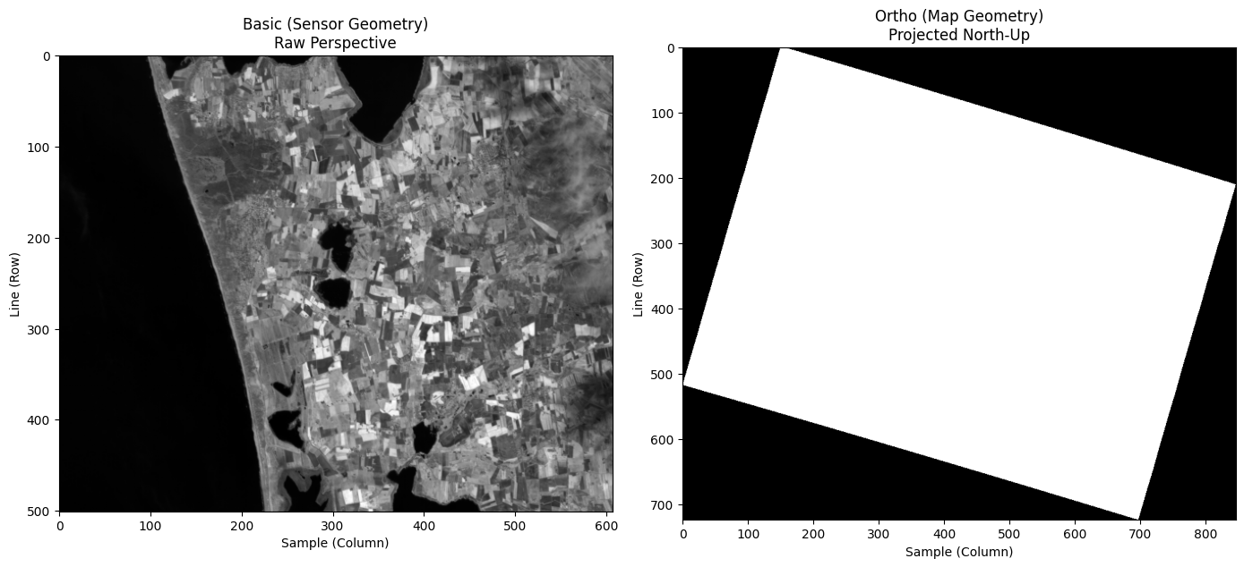
What went wrong?
If you look at the output, the Basic image (left) looks fine, but the Ortho image (right) likely appears as a solid white shape on a black background. You can’t see the land cover or surface details. Is the file empty?
No. The problem is the fill value (no-data).
What’s going on?
Geometry: Orthorectification rotates the swath to fit a projected map grid. That creates empty corners (areas outside the imaged footprint).
Fill value: In remote sensing, these empty areas are filled with a value like
-9999so software can identify them as “no data.” Tanager-1 follows this convention.The calculation: When imshow auto-scaled the display range using the minimum and maximum pixel values, Python used all pixels, including the
-9999fill values. The stretch range became[-9999, 0.3]. On that scale, real reflectance values (0.01–0.3) cluster at the top and appear as pure white.
How can we fix this?
We need to mask the fill value (-9999) so Python excludes those pixels when computing statistics and visualization. That way, calculations are based only on real reflectance data, and the Ortho image will display correctly.
Best practice: Before masking, plot a histogram of the band to inspect the distribution. Let’s plot and see!
# plot histogram for Ortho Slice

plt.figure(figsize=(10, 5))
plt.hist(ortho_slice.flatten(), bins=100, edgecolor='black', alpha=0.7)
plt.xlabel('Surface Reflectance')
plt.ylabel('Pixel Count')
plt.title(f'Ortho Band {band_number} Distribution')
plt.grid(True, alpha=0.3)
plt.show()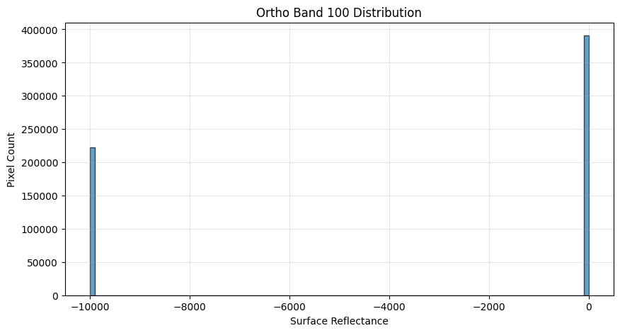
You see the fill-value spike at -9999, and there’s also a spike around zero (valid reflectance values). Let’s mask -9999 as np.nan and see what the histogram looks like.
# replace -9999 with np.nan
ortho_slice[ortho_slice == -9999] = np.nan
# Replot the histogram after removing `-9999` values
plt.figure(figsize=(10, 5))
plt.hist(ortho_slice.flatten(), bins=100, edgecolor='black', alpha=0.7)
plt.xlabel('Surface Reflectance')
plt.ylabel('Pixel Count')
plt.title(f'Ortho Band {band_number} Distribution')
plt.grid(True, alpha=0.3)
plt.show()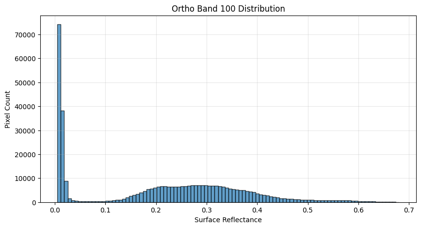
Now, we can compare the Basic and Ortho assets and see the difference.
# Create side-by-side figure: unpack axes as (Basic, Ortho) for clarity
fig, (basic, ortho) = plt.subplots(1, 2, figsize=(14, 8))

# Left: Basic (sensor geometry)
basic.imshow(basic_slice, cmap='gray')
basic.set_title("Basic (Sensor Geometry)\nRaw Perspective")
basic.set_xlabel("Sample (Column)")
basic.set_ylabel("Line (Row)")

# Right: Ortho (map geometry)
ortho.imshow(ortho_slice, cmap='gray')
ortho.set_title("Ortho (Map Geometry)\nProjected North-Up")
ortho.set_xlabel("Sample (Column)")
ortho.set_ylabel("Line (Row)")

plt.tight_layout()
plt.show()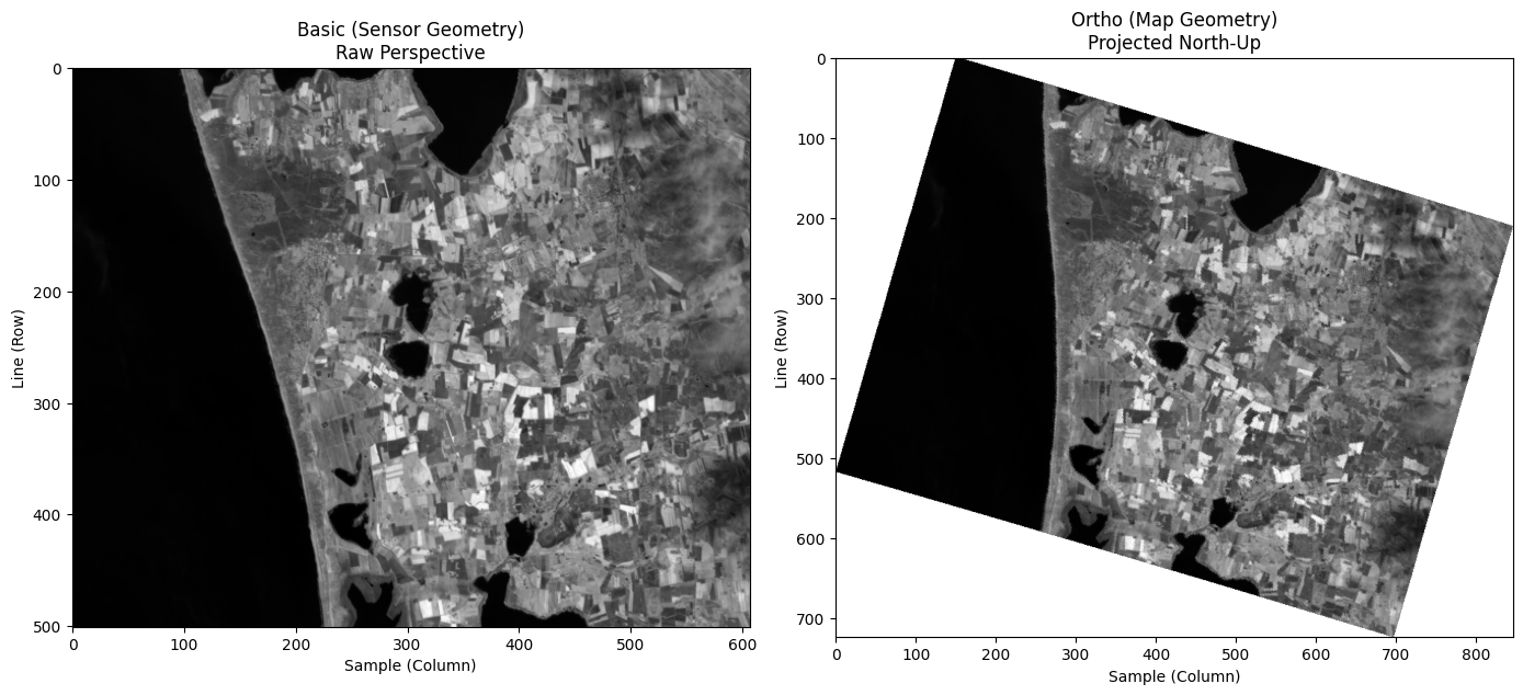
Now you can see both assets!
Now that both images display correctly, look closely at the side-by-side comparison. Same patch of Earth, two very different views.
Key Difference: Raw Perspective vs. Geometric Correction
Basic: Features like roads, lakes, or agricultural fields may appear warped, compressed, or skewed. Why: The sensor is capturing data at an angle and over uneven terrain. A higher (i.e., more off-nadir) viewing angle or elevation changes on the ground may distort how the shapes are captured by the detectors.
Ortho: The features are geometrically corrected and true to their real-world shapes. Why: The orthorectification pipeline uses a DEM (Digital Elevation Model) to correct for “relief displacement”, ironing out the distortions caused by topography and sensor viewing angles. A square field on the ground now maps as a perfect square in the image, allowing it to be seamlessly overlaid with standard maps or vector data.
Summary & Next Steps
You’ve compared Basic and Ortho assets side-by-side and seen how geometry transforms from the raw sensor swath to a map-projected grid. Understanding when to use each format is essential for building robust analysis pipelines.
Next Up: In Lesson 4 of Module 2, we’ll dive into the physics of light, comparing Radiance vs Surface Reflectance and learning the differences.
See you in Lesson 4 of Module 2: Radiance vs Reflectance!