
Welcome to the first lesson of the TanagerSpec module. In this lesson, we will introduce you to setting up and initializing the TanagerSpec package. This foundational workflow establishes the core pattern you will repeat across all coming lessons—the object → accessor → method call shape defined in the section How TanagerSpec Method Calls Are Structured below.
Installing TanagerSpec
Setting up TanagerSpec is quick and straightforward!
You have two simple options to get started:
Option 1: Install from PyPI (Recommended)
TanagerSpec is published on PyPI.
Open a terminal in your Python environment and run:
pip install tanagerspecOption 2: Install from Source (Manual Install)
If you want the latest development version or plan to contribute, you can install TanagerSpec from the source code:
Clone the repository from GitHub:
git clone https://github.com/planetlabs/tanagerspec.gitNavigate to the cloned directory:
cd tanagerspecInstall the package using pip:
pip install .
Now you’re ready to use TanagerSpec in your analysis workflows!
## Unhide cell for package install if needed

# %pip install tanagerspec
Get Tanager Scene (Download Data)
TanagerSpec provides helpful utilities that enhance the experience of working with hyperspectral data. In this lesson, we will start by using one of them: download_scene. This tool allows you to quickly download a Tanager-1 scene and store its file path in a variable, which can then be used to initialize your workflow.
To run the steps below, you will need the URL of your scene of interest from the Open STAC catalog.
Organizing Our Workspace
Before downloading a hyperspectral dataset, it is best practice to establish a clean folder structure. Setting up our directories first achieves two main goals:
Keeps the root directory clean: We route raw downloaded files into a dedicated
data/folder.Prevents accidental overwrites: We create an
outputs/folder tagged with the current date and hour. If you run this notebook multiple times or process different scenes, your previous outputs (like plots or processed data) will remain safe from being overwritten.
from pathlib import Path
from datetime import datetime

DATA_DIR = Path("data")
DATA_DIR.mkdir(parents=True, exist_ok=True)

timestamp = datetime.now().strftime("%Y%m%d_%H")
OUTPUT_DIR = Path(f"outputs_{timestamp}")
OUTPUT_DIR.mkdir(parents=True, exist_ok=True)
Downloading the Scene
Now that our file structure is ready, we can download the scene directly into our data folder. We will pass the scene’s URL and our target destination path to the download_scene function.
from tanagerspec import download_scene

URL = "https://storage.googleapis.com/open-cogs/planet-stac/tanager1-release2-core-imagery/ortho_sr_hdf5/20250501_143138_87_4001_ortho_sr_hdf5.h5"
FILE_NAME = "ortho_sr_scene.h5"

TANAGER_SCENE_PATH = download_scene(
    URL,
    DATA_DIR / FILE_NAME
)

if TANAGER_SCENE_PATH is not None and Path(TANAGER_SCENE_PATH).exists():
    print(f"Scene downloaded successfully to: {TANAGER_SCENE_PATH}")
else:
    print("Scene download failed or file does not exist.")
Inspecting the HDF5 Scene Structure
Now that our file is successfully downloaded, let’s explore its contents using another helpful TanagerSpec utility: inspect_hdf.
Data formatted in HDF5-EOS acts like an internal file system containing nested groups and datasets. If you want to perform custom analyses, extract specific spectral bands, or pull out ancillary metadata, you will need to know exactly where they live inside the file.
The inspect_hdf function provides a clean, readable overview of this internal hierarchy, making it easy to find and copy the exact internal paths you need for your custom workflows.
from tanagerspec import inspect_hdf

inspect_hdf(TANAGER_SCENE_PATH)
Inspecting HDF file: /Users/abdelrahman.saleh/Desktop/Hyperspec development/hyperspec/notebooks/new tutorial/data/ortho_sr_ag_scene.h5
📂 HDFEOS/
📂 HDFEOS/ADDITIONAL/
📂 HDFEOS/ADDITIONAL/FILE_ATTRIBUTES/
📂 HDFEOS/GRIDS/
📂 HDFEOS/GRIDS/HYP/
↳ 🏷️ created_at: 2025-12-05T23:21:42.763982+00:00
↳ 🏷️ epsg_code: 32721
↳ 🏷️ strip_id: 20250501_143134_00_4001_strip
📂 HDFEOS/GRIDS/HYP/Data Fields/
📄 HDFEOS/GRIDS/HYP/Data Fields/aerosol_optical_depth | (752, 784) | float32
↳ 🏷️ Unit: Unitless
↳ 🏷️ _FillValue: -9999.0
📄 HDFEOS/GRIDS/HYP/Data Fields/beta_cirrus_mask | (752, 784) | uint8
↳ 🏷️ _FillValue: 255
📄 HDFEOS/GRIDS/HYP/Data Fields/beta_cloud_mask | (752, 784) | uint8
↳ 🏷️ _FillValue: 255
📄 HDFEOS/GRIDS/HYP/Data Fields/column_water_vapour | (752, 784) | float32
↳ 🏷️ Unit: g/cm^2
↳ 🏷️ _FillValue: -9999.0
📄 HDFEOS/GRIDS/HYP/Data Fields/nodata_pixels | (752, 784) | uint8
↳ 🏷️ _FillValue: 255
📄 HDFEOS/GRIDS/HYP/Data Fields/sensor_azimuth | (752, 784) | float32
↳ 🏷️ Unit: Decimal Degrees
↳ 🏷️ _FillValue: -9999.0
📄 HDFEOS/GRIDS/HYP/Data Fields/sensor_to_ground_path_length | (752, 784) | float32
↳ 🏷️ Unit: Meters
↳ 🏷️ _FillValue: -9999.0
📄 HDFEOS/GRIDS/HYP/Data Fields/sensor_zenith | (752, 784) | float32
↳ 🏷️ Unit: Decimal Degrees
↳ 🏷️ _FillValue: -9999.0
📄 HDFEOS/GRIDS/HYP/Data Fields/sun_azimuth | (752, 784) | float32
↳ 🏷️ Unit: Decimal Degrees
↳ 🏷️ _FillValue: -9999.0
📄 HDFEOS/GRIDS/HYP/Data Fields/sun_zenith | (752, 784) | float32
↳ 🏷️ Unit: Decimal Degrees
↳ 🏷️ _FillValue: -9999.0
📄 HDFEOS/GRIDS/HYP/Data Fields/surface_reflectance | (426, 752, 784) | float32
↳ 🏷️ Unit: Unitless
↳ 🏷️ _FillValue: -9999.0
↳ 🏷️ fwhm: [5.39 5.42 5.45 5.48 5.52 5.55 5.58 5.6 5.63 5.66...
↳ 🏷️ fwhm_units: nm
↳ 🏷️ good_wavelengths: [1 1 1 1 1 1 1 1 1 1 1 1 1 1 1 1 1 1 1 1 1 1 1 1 1...
↳ 🏷️ wavelengths: [ 376.44 381.41 386.38 391.35 396.32 401.29 ...
↳ 🏷️ wavelengths_units: nm
📄 HDFEOS/GRIDS/HYP/Data Fields/surface_reflectance_uncertainty | (426, 752, 784) | float32
↳ 🏷️ Unit: Unitless
↳ 🏷️ _FillValue: -9999.0
📄 HDFEOS/GRIDS/HYP/Data Fields/time | (752, 784) | float64
↳ 🏷️ Unit: UTC
↳ 🏷️ _FillValue: -9999.0
📂 HDFEOS INFORMATION/
↳ 🏷️ HDFEOSVersion: b'HDFEOS_5.1.15'
📄 HDFEOS INFORMATION/StructMetadata.0 | () | |S32000
Initialize TanagerSpec and Load the Data
After downloading our file and inspecting its internal structure, we’re ready to load the HDF5 data into a TanagerSpec object. This object will become our primary interface for all subsequent hyperspectral analysis, visualization, and manipulation.
To do this, we use the .from_file() method. By specifying the file path and setting the loader as "TanagerLoader", TanagerSpec takes care of reading and parsing the complex HDF5 structure for us.
from tanagerspec import TanagerSpec

tanager_ortho_sr = TanagerSpec.from_file(TANAGER_SCENE_PATH)
print("TanagerSpec object successfully initialized!")
How TanagerSpec Method Calls Are Structured
Once your scene is loaded into a TanagerSpec object, almost every analysis step follows the same fluent call shape:
result = tanager_cube.<accessor>.<method>(...)For example:
tanager_ortho_sr.plot.rgb(...)
tanager_ortho_sr.preprocess(...)
tanager_ortho_sr.analysis.compare_bands(...)
Anatomy of a Method Call
Every method call shares the same skeleton. Parameters are usually grouped by purpose, spectral selection, scaling, and export, even when the exact keyword names change from method to method:
#  Output    Object   accessor   Method
#   │          │          │        │
#   ▼          ▼          ▼        ▼
   result = tanager_cube.plot.some_method(
       # --- spectral / analysis options ---
       ...,
       # --- display & export controls (common across many methods) ---
       plot=True,
       save_png=FIGURE_DIR / "example.png",
   )
💡 Core TanagerSpec Design Pattern: Always Capture Outputs Most
.plot.*and.analysis.*calls return underlying data, NumPy arrays, dictionaries, or file paths, not just figures. Assign the result to a variable when you need to reuse it downstream (custom maps, machine learning, exports) without recomputing.
Where You Will See Each Accessor
| Accessor | Role in later lessons |
|---|---|
.plot | RGB composites, band galleries, spectra, animation (Lesson 18) |
Chain methods (e.g. .drop_bands(), .preprocess(), .denoise()) | Masks, clipping, denoise (Lesson 16) |
.convert_to | GeoTIFF, ENVI, xarray export (Lesson 17) |
.analysis | Band compare, indices, ML (Lessons 18–21) |
In later notebooks we show what each method does. This lesson shows how calls are shaped so you can read any example at a glance.
Organizing Your Project Directory
As you work with TanagerSpec, you will generate various outputs such as figures, processed data, and analysis results. Because TanagerSpec provides the flexibility to specify exactly where your outputs are saved, it is highly recommended to establish an organized directory structure from the start.
Instead of saving everything into a single main OUTPUT_DIR, creating dedicated subfolders for different steps in your workflow (e.g., plots, exported rasters, or machine learning results) is a great practice. This approach keeps your workspace tidy and ensures you can easily locate specific files later. Here, we will demonstrate this workflow by first setting up a dedicated folder specifically for our output plots and figures before we begin saving.
Now that we understand the importance of organizing our workspace, let’s put it into practice. We will use Python’s built-in path handling to create a new folder named figures inside our main OUTPUT_DIR.
FIGURE_DIR = OUTPUT_DIR / "figures"
FIGURE_DIR.mkdir(parents=True, exist_ok=True)

print(f"Figures will be saved to: {FIGURE_DIR}")
Quick note: OUTPUT_DIR / "figures" joins paths cleanly; parents=True creates missing parent folders; exist_ok=True avoids errors if you re-run the cell.
Exploring Scene Metadata
Now that our data is loaded into the tanager_ortho_sr object, we can use its built-in .info() method to get a quick, comprehensive summary of the scene.
Your First Method Call: .info()
The cell below is a concrete example of the call pattern introduced above:
tanager_ortho_sr— your loaded cube object.info(...)— a method on that object (core introspection; no accessor prefix needed)save_png=FIGURE_DIR / "..."— an export keyword you will see again on.plot.*methods lesson.
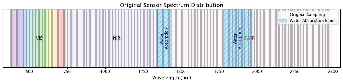
Calling .info() extracts essential metadata directly from the loaded file, giving you an immediate snapshot of the image dimensions, total spectral bands, wavelength ranges, and spatial referencing.
Understanding Tanager Product Types
One key piece of information to look for in your summary is the Product Type. The TanagerSpec package is designed to work seamlessly with two different surface reflectance (sr) data formats:
ortho_sr(Orthorectified)basic_sr(Basic)
Let’s run the cell below to inspect our scene and save the output:
tanager_ortho_sr.info(
    save_png=FIGURE_DIR / "ortho_sr_info.png"
)
==================================================
Hyperspectral Dataset Information
==================================================
Product Type: ortho_sr
Shape: (426, 752, 784)
Number of Bands: 426
Wavelength Range: 376.44 - 2499.00 nm
Data Type: float32
CRS: EPSG:32721
Transform: | 30.00, 0.00, 699630.00|
| 0.00,-30.00, 8301180.00|
| 0.00, 0.00, 1.00|
Bands Dropped: False
Denoised: False
==================================================
Band status figure saved to outputs_20260501_013832/figures/ortho_sr_info.png
Visualizing the Spectrum Distribution
Notice that calling .info() also generates a visual layout of your sensor’s spectral sampling alongside the text summary.
In this visualization, you can see the complete distribution of the 426 bands across the Visible (VIS), Near-Infrared (NIR), and Shortwave-Infrared (SWIR) regions, along with shaded areas highlighting the standard atmospheric water-absorption bands.
These shaded regions, most prominently near 1400 nm and 1900 nm are wavelengths where water vapour in the atmosphere absorbs almost all of the incoming and reflected light. Very little signal reaches the sensor there, so the surface-reflectance estimate in those bands is unreliable and noisy. You will routinely exclude these bands before analysis, which is exactly what the next lesson on preprocessing covers.
It is highly recommended to treat .info() as your primary diagnostic tool to verify the state of your hyperspectral data throughout your analysis.
In our current summary, notice the field at the bottom:
Bands Dropped: FalseIn the next lesson on Preprocessing, we will learn how to use built-in methods to drop noisy bands from our analysis. When you apply these methods, running .info() again will dynamically update to reflect your changes. The Bands Dropped field will change to list the wavelengths of the dropped bands, the total band count will decrease, and the output visualization chart will automatically adjust to show exactly which wavelengths were removed from your dataset.
What’s Next?
You have successfully downloaded, organized, and loaded your Tanager scene, and you now know how to inspect its metadata and spectral layout. Your workspace is perfectly prepped and ready for action.
Before you can analyze hyperspectral scenes, it’s important to properly clean and prepare your data. In the next lesson, Preprocessing, we will explore how TanagerSpec simplifies this workflow. You will learn how to:
Exclude Unwanted Bands: Easily drop noisy or unneeded wavelength regions.
Apply Quality Masks: Filter out invalid or poor-quality pixels.
Clip Reflectance Values: Ensure your data stays within valid physical boundaries.
Reduce Noise: Apply automated denoising to clean up your signal.
By the end of the next lesson, you will ensure your data is highly reliable and fully optimized for downstream analysis.
See you in the next lesson!