Welcome to Lesson 1 of Module 1 (Mission & Foundation). Before diving into the hands-on work, it’s important to understand the instrument and mission behind the data we’ll be using.
In this short lesson, you’ll get an introduction to Planet’s Tanager mission and a concise overview of the key technical specifications that will come up again throughout this course.
Objectives:
Understand the Tanager mission and its significance for Earth Observation
Learn Tanager’s key technical specifications.
Familiarize yourself with TanagerScene asset types and file formats
Note: Objectives 2 and 3 are explored in depth in Module 2. Here, we provide a brief overview so you have a foundation before diving into the details.
Mission Overview: Why Hyperspectral Matters
Tanager-1 is the first satellite in Planet’s hyperspectral constellation. This constellation has its roots in the Carbon Mapper Coalition, a public-private partnership bringing together Carbon Mapper, Inc., Planet Labs, PBC and NASA Jet Propulsion Laboratory as the main technology and science partners. While Tanager’s headline mission is detecting large methane and carbon dioxide emissions, it is more than a methane satellite. Tanager’s full VSWIR spectral range means it provides a massive volume of “Core Imagery” that is invaluable for many Earth Observation (EO) applications, unlocking new capabilities for agriculture, mineralogy, and water quality monitoring.
The Hyperspectral Advantage
Most commonly used multispectral satellites (like Landsat or Sentinel-2) measure light in approximately 10–13 broad, disconnected bands. These bands are placed to capture general information about the surface, but they lack the spectral resolution to discern subtle details and differences found across the spectral range.
Tanager-1 changes the paradigm by capturing a continuous spectrum. Instead of averaging light over wide ranges, it records the reflected energy in hundreds of narrow, contiguous channels. This density of information allows you to resolve narrow absorption features, specific dips in the spectrum caused by chemical bonds (like chlorophyll, cellulose, or specific minerals), that broadband sensors simply can’t see. It also capture the full picture of how energy in each narrow wavelength interacts with the atmosphere and surface over the entire VSWIR spectral range.
This capability turns standard imagery into spectroscopy, allowing you to identify the unique “spectral fingerprint” of materials on the ground rather than just their general informations.
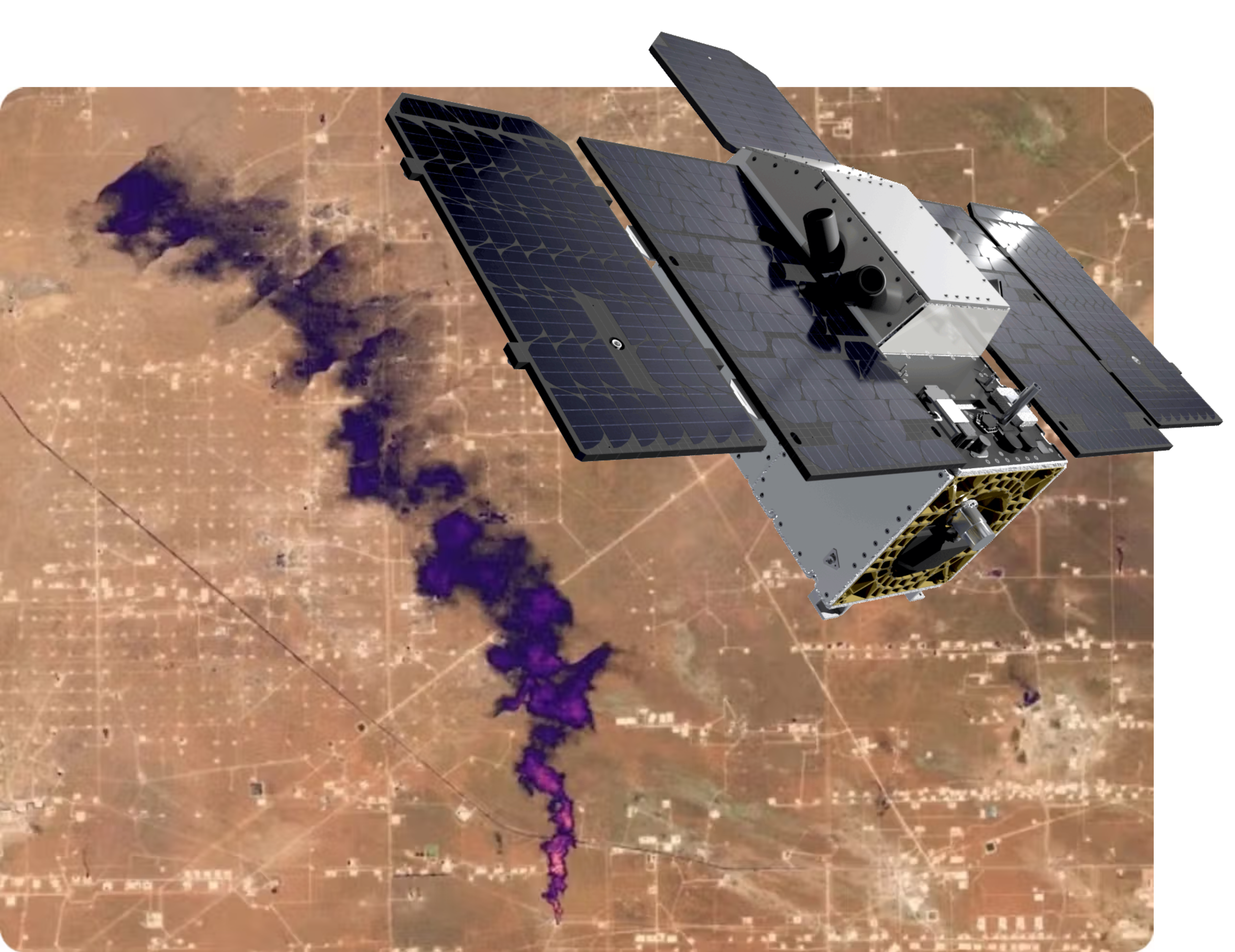
Tanager-1 satellite.
Data Product Overview and Technical Specifications
To achieve this continuous spectral capture, Tanager-1 uses a specialized instrument architecture that differs significantly from standard cameras.
Instrument Architecture
The satellite carries a VSWIR (Visible to Shortwave Infrared) imaging spectrometer that operates as a line-scanner. Unlike a frame camera that snaps a square photo, Tanager builds an image line-by-line as it orbits, collecting data across the full 376–2500 nm range.
Spectral Bands: ~426 contiguous bands
Spectral Sampling: ~5 nm (allowing us to resolve fine spectral features)
Radiometry: Data is delivered as either:
Calibrated Radiance (TOA): Energy measured at the sensor (Top-of-Atmosphere) in units of calibrated radiance. Scattering and absorption by the atmosphere is present in these measurements. Surface Reflectance (BOA): The proportion of incoming light that gets reflected, transmitted, or emitted from the ground (Bottom-of-Atmosphere). This product has been atmospherically corrected to remove haze, water vapor, and aerosols, making it the standard for most surface analyses.
Geometry: Basic and Ortho Scenes
Planet provides two geometry types for Tanager imagery. Choosing the right one for your work depends on your application and analysis methods.
Basic Scene (Sensor Geometry)
Basic products contain the hyperspectral data cube in sensor or image space.
The “Why”: Scientists often prefer to work with Basic scenes because they contain the data as measured by the instrument. No spatial resampling or interpolation has been applied to fit the data to a 2-D projection or map grid, preserving the original spectral integrity. Scientists usually project the results of their spectral analysis after doing the processing in sensor space. For example, you may apply a mineral detection algorithm and then project the resulting mineral presence or abundance map to a specific map grid.
The Trade-off: Each pixel in a Basic image has been georeferenced with its latitude and longitude in the WGS84 Geographic Coordinate System (GCS). This information is provided in the Geolocation Arrays in the assets. However, because the Basic data cube hasn’t been projected, you cannot overlay it directly on a map or onto other projected data layers. You can use your own Digital Elevation Model to project the data into any map grid you desire with your own selection of resampling kernel.
Ortho Scene (Map Geometry)
Ortho products have been orthorectified (corrected for terrain and sensor geometry) and projected to a map grid (UTM).
The “Why”: This is “Analysis Ready Data” for most GIS users. It overlays onto other projected raster images and feature maps (like roads or field boundaries).
The Trade-off: The pixel values have been resampled to fit the grid, using Nearest Neighbor resampling. This means there is no spectral interpolation, and measured spectra are preserved in the Ortho product. BUT native Tanager Ground Sampling Distance is often slightly coarser than the 30 m grid we use for our Ortho products. Nearest Neighbor resampling means that there will be many redundant spectra in the Ortho data cubes, and users may notice geometric impacts like aliasing.
File Format: HDF-EOS5
Both Basic and Ortho assets are delivered in HDF-EOS5 (HDF5) format.
Think of HDF5 as a “FileSystem in a File”: unlike a GeoTIFF (which is usually just one image), an HDF5 file contains a hierarchy of folders (“Groups”) and data (“Datasets”) all inside one file.
It is Self-describing (metadata is stored inside).
It allows Partial Reading (you can load just the Green band without loading the whole 10GB file).
⚠️ Note: Since this hierarchical format is more complex than standard GeoTIFFs, the next lessons will focus on building your skills to navigate it with Python.
Table 1. Tanager-1 Technical Specifications (Quick Reference)
| Feature | Specification | Notes |
|---|---|---|
| Spectral Range | 376 – 2500 nm | Visible to Shortwave Infrared (VSWIR) |
| Spectral Bands | ~426 bands | Contiguous spectral sampling |
| Spectral Sampling | ~5 nm | FWHM / Bandwidth ~5.2-6.8 nm |
| Ground Sample Distance | ~32 m (at Nadir) | Varies by altitude & view angle |
| Pixel Size (Ortho) | 30 m | Standard grid size for analysis |
| Swath Width | ~18 km | Narrow swath (approx. 600 pixels wide) |
| Revisit Rate | Variable | Targeted tasking (not a continuous mapper) |
References
The sources for this lesson are:
For more detailed and up-to-date technical information, please refer back to these sources.
Summary & Next Steps
You’ve now completed the introduction to the Tanager Hyperspectral Mission. In the next lessons, we’ll shift from mission context to hands-on skills, building the foundation you need to confidently open, explore, and work with HDF5 (HDF-EOS5) files.
See you in Lesson 2 of Module 1!