This course is organized into five modules. We start by understanding the mission and how Tanager data is stored (Module 1), then learn what the products mean physically (Module 2). Next, we prepare clean, analysis-ready inputs (Module 3), and apply real hyperspectral workflows and analysis techniques like spectral indices, dimension reduction, and machine learning (ML), to produce insight and maps (Module 4). Finally, Module 5 brings everything together through TanagerSpec, Planet Labs’ integrated Python package that unifies the entire workflow into a single, streamlined toolkit. The course’s path is illustrated in Figure 1.
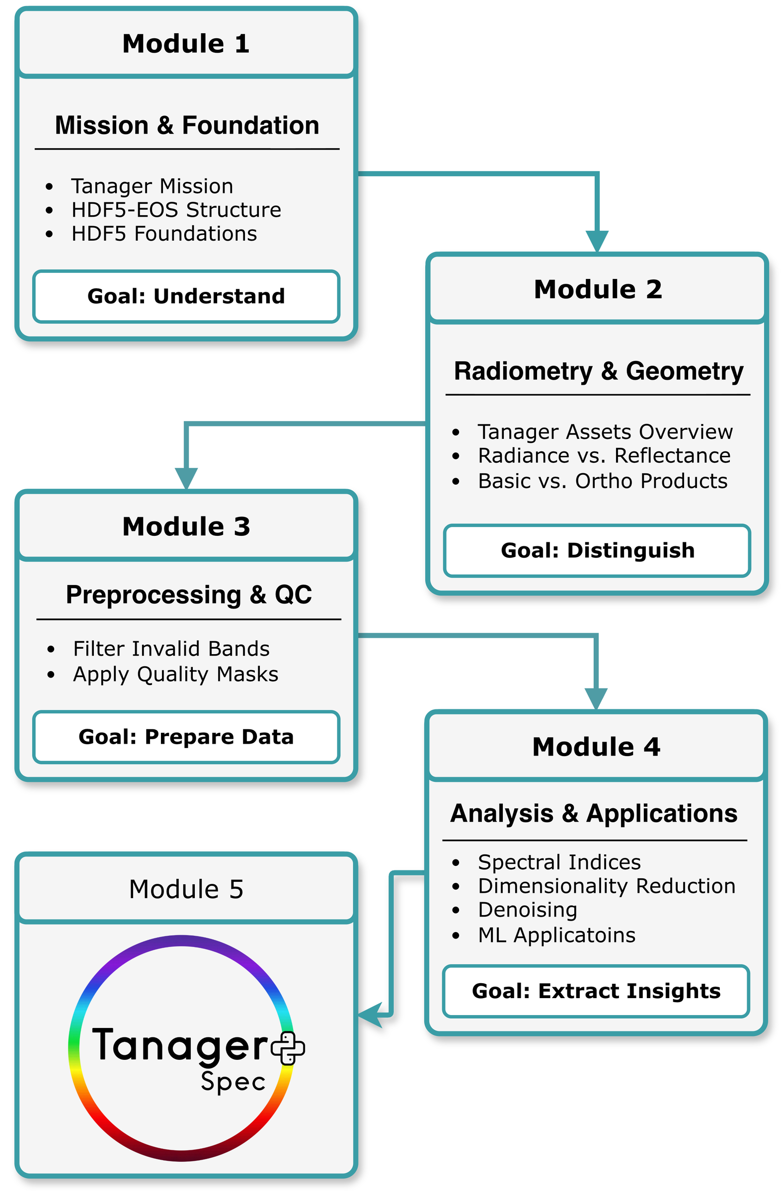
Figure 1:Tanager: Hyperspectral Data Analysis Course Path
Module 1: Mission & Foundation (The Container)
This module establishes the foundations of the Tanager mission. You’ll start with the mission and instrument at a high level, then build a practical understanding of the HDF5-EOS file structure used in Tanager data products.
Because this format can feel complex at first, you’ll learn it step by step by building an HDF5 file from scratch. This gives you “X-ray vision” into how groups, datasets, attributes, and metadata are organized, so you can confidently navigate real Tanager files.
You will produce:
A small HDF5 file you created from scratch (for structure intuition)
A “Tanager file map” notebook that can locate key datasets and metadata
Transition: Once you can navigate the container, we move to the meaning of what’s inside it—radiometry and geometry.
Module 2: Radiometry & Geometry (The Physics)
In this module you’ll learn the two key layers behind Tanager products: radiometry (radiance vs. surface reflectance) and geometry (basic vs. ortho). You’ll work with real .h5 files and learn how to choose the right product for your task.
Each Tanager scene is delivered as an ecosystem of seven assets. By the end of this module, you’ll be able to identify each asset, understand its role, and clearly distinguish between: Radiance vs. Reflectance and Basic vs. Ortho products.
You will produce: a simple decision guide for choosing Radiance vs. SR and Basic vs. Ortho, plus the supporting assets you need (UDM + geolocation).
Transition: Once you understand the products and their meaning, the next step is ensuring the data is clean and consistent for analysis.
Module 3: Preprocessing & Quality Control (The Bridge)
This short “bridge” module connects product understanding to real analysis. The goal is to ensure your inputs are clean, consistent, and analysis-ready before you move into applications.
You’ll learn core hyperspectral preprocessing steps to produce an analysis-ready hyperspectral cube, including:
Removing unusable or noisy bands
Masking and handling invalid pixels to standardize data quality
You will produce:
An analysis-ready hyperspectral cube
A QC summary (e.g., how many bands removed, how many pixels masked, basic sanity plots)
Transition: Now that your cube is analysis-ready, we can use it to generate insight, maps, and quantitative results.
Module 4: Analysis & Applications (The Insight)
This final module brings everything together. You’ll use the analysis-ready hyperspectral cube from Module 3 to turn spectral measurements into actionable insights. The emphasis is on practical hyperspectral workflows used in real projects: indices, machine learning, and quantification.
You’ll extract information from spectra through three key steps:
Narrowband spectral indices (fast insights) Compute optimized narrowband indices that leverage hyperspectral detail (specific wavelengths rather than broad multispectral-style bands) to characterize targets such as vegetation and water.
Dimensionality reduction (efficient and robust analysis) Address the curse of dimensionality by summarizing information across “all those bands” and improve model stability using reduction methods, starting with Principal Component Analysis (PCA).
Applications & quantification (maps and estimates) Move from exploration to prediction by applying:
Unsupervised learning for pattern discovery (e.g., clustering for scene segmentation)
Supervised classification to map classes of interest (e.g., Random Forest)
Regression (quantification) to estimate continuous variables from spectra
You will produce:
Index maps and interpretive plots
PCA outputs (components, variance explained, feature-space visualizations)
ML outputs (classification maps and/or regression estimates)
Transition: Now that you’ve mastered core analysis techniques, Module 5 shows you how to execute the same workflows more efficiently using TanagerSpec’s integrated toolkit.
Module 5: TanagerSpec — Putting It All Together (The Toolkit)
This module introduces TanagerSpec, Planet Labs’ purpose-built Python package for Tanager hyperspectral analysis. After building individual skills across Modules 1–4, you’ll use TanagerSpec to unify them into a coherent, end-to-end workflow with an intuitive, integrated interface.
Sub-lessons:
Orientation and Initialization — install TanagerSpec, download data via Open STAC, and read scene metadata
Preprocessing — quality masking, reflectance clipping, band exclusion, and denoising
Export and Conversion — convert HDF5-EOS files to GeoTIFF and ENVI-BIL
Visualization and Exploration — quick scene inspection, band exploration, and spectral signature comparison
Spectral Indices — built-in catalog of 200+ ready-to-use indices spanning vegetation, water, soils, urban, snow, and burn severity
Index Creator Lab — design custom spectral indices tailored to your own objectives and experiments
Machine Learning Applications — dimensionality reduction, clustering, spectral library construction, and classification
You will produce:
Visual products (RGB composites, band images, spectral signature plots)
Index maps from the built-in catalog and custom-designed indices
Clustered and classified scene maps
Exported GeoTIFF / ENVI files ready for GIS and remote sensing workflows
Prerequisites and Requirements
To get the most out of this course, you should be comfortable running Python notebooks and have a basic foundation in array-based computing and plotting. Don’t worry if you’re not fully confident, following the lessons step by step will help you build confidence in your coding skills. We also encourage you to use AI tools whenever something feels unclear.
Prerequisites:
Fundamentals of remote sensing (preferred)
Basic Python programming:
Variables
Functions
Loops
Dictionaries
Familiarity with NumPy
Familiarity with Matplotlib
Minimum: 16 GB RAM, 20 GB free storage